case control studies disadvantages

Case-Control Studies

•   1  
• |   2  
• |   3  
• |   4  
• |   5  
• |   6  
• |   7  
• |   8  

E pi_Tools.XLSX

All Modules

Advantages and Disadvantages of Case-Control Studies

Advantages:

• They are efficient for rare diseases or diseases with a long latency period between exposure and disease manifestation.
• They are less costly and less time-consuming; they are advantageous when exposure data is expensive or hard to obtain.
• They are advantageous when studying dynamic populations in which follow-up is difficult.

Disadvantages:

• They are subject to selection bias.
• They are inefficient for rare exposures.
• Information on exposure is subject to observation bias.
• They generally do not allow calculation of incidence (absolute risk).

When is it desirable to use a case-control study?

a.  When the disease is rare.

b.  When the study population is dynamic.

c.  When the disease has a long latency period.

d.  When studying multiple health effects (diseases) stemming from a single exposure.

return to top | previous page

Content ©2016. All Rights Reserved. Date last modified: June 7, 2016. Wayne W. LaMorte, MD, PhD, MPH

Have a language expert improve your writing

Run a free plagiarism check in 10 minutes, generate accurate citations for free.

• Knowledge Base

Methodology

• What Is a Case-Control Study? | Definition & Examples

What Is a Case-Control Study? | Definition & Examples

Published on February 4, 2023 by Tegan George . Revised on June 22, 2023.

A case-control study is an experimental design that compares a group of participants possessing a condition of interest to a very similar group lacking that condition. Here, the participants possessing the attribute of study, such as a disease, are called the “case,” and those without it are the “control.”

It’s important to remember that the case group is chosen because they already possess the attribute of interest. The point of the control group is to facilitate investigation, e.g., studying whether the case group systematically exhibits that attribute more than the control group does.

Table of contents

When to use a case-control study, examples of case-control studies, advantages and disadvantages of case-control studies, other interesting articles, frequently asked questions.

Case-control studies are a type of observational study often used in fields like medical research, environmental health, or epidemiology. While most observational studies are qualitative in nature, case-control studies can also be quantitative , and they often are in healthcare settings. Case-control studies can be used for both exploratory and explanatory research , and they are a good choice for studying research topics like disease exposure and health outcomes.

A case-control study may be a good fit for your research if it meets the following criteria.

• Data on exposure (e.g., to a chemical or a pesticide) are difficult to obtain or expensive.
• The disease associated with the exposure you’re studying has a long incubation period or is rare or under-studied (e.g., AIDS in the early 1980s).
• The population you are studying is difficult to contact for follow-up questions (e.g., asylum seekers).

Retrospective cohort studies use existing secondary research data, such as medical records or databases, to identify a group of people with a common exposure or risk factor and to observe their outcomes over time. Case-control studies conduct primary research , comparing a group of participants possessing a condition of interest to a very similar group lacking that condition in real time.

Prevent plagiarism. Run a free check.

Case-control studies are common in fields like epidemiology, healthcare, and psychology.

You would then collect data on your participants’ exposure to contaminated drinking water, focusing on variables such as the source of said water and the duration of exposure, for both groups. You could then compare the two to determine if there is a relationship between drinking water contamination and the risk of developing a gastrointestinal illness. Example: Healthcare case-control study You are interested in the relationship between the dietary intake of a particular vitamin (e.g., vitamin D) and the risk of developing osteoporosis later in life. Here, the case group would be individuals who have been diagnosed with osteoporosis, while the control group would be individuals without osteoporosis.

You would then collect information on dietary intake of vitamin D for both the cases and controls and compare the two groups to determine if there is a relationship between vitamin D intake and the risk of developing osteoporosis. Example: Psychology case-control study You are studying the relationship between early-childhood stress and the likelihood of later developing post-traumatic stress disorder (PTSD). Here, the case group would be individuals who have been diagnosed with PTSD, while the control group would be individuals without PTSD.

Case-control studies are a solid research method choice, but they come with distinct advantages and disadvantages.

Advantages of case-control studies

• Case-control studies are a great choice if you have any ethical considerations about your participants that could preclude you from using a traditional experimental design .
• Case-control studies are time efficient and fairly inexpensive to conduct because they require fewer subjects than other research methods .
• If there were multiple exposures leading to a single outcome, case-control studies can incorporate that. As such, they truly shine when used to study rare outcomes or outbreaks of a particular disease .

Disadvantages of case-control studies

• Case-control studies, similarly to observational studies, run a high risk of research biases . They are particularly susceptible to observer bias , recall bias , and interviewer bias.
• In the case of very rare exposures of the outcome studied, attempting to conduct a case-control study can be very time consuming and inefficient .
• Case-control studies in general have low internal validity  and are not always credible.

Case-control studies by design focus on one singular outcome. This makes them very rigid and not generalizable , as no extrapolation can be made about other outcomes like risk recurrence or future exposure threat. This leads to less satisfying results than other methodological choices.

If you want to know more about statistics , methodology , or research bias , make sure to check out some of our other articles with explanations and examples.

• Student’s  t -distribution
• Normal distribution
• Null and Alternative Hypotheses
• Chi square tests
• Confidence interval
• Quartiles & Quantiles
• Cluster sampling
• Stratified sampling
• Data cleansing
• Reproducibility vs Replicability
• Peer review
• Prospective cohort study

Research bias

• Implicit bias
• Cognitive bias
• Placebo effect
• Hawthorne effect
• Hindsight bias
• Affect heuristic
• Social desirability bias

A case-control study differs from a cohort study because cohort studies are more longitudinal in nature and do not necessarily require a control group .

While one may be added if the investigator so chooses, members of the cohort are primarily selected because of a shared characteristic among them. In particular, retrospective cohort studies are designed to follow a group of people with a common exposure or risk factor over time and observe their outcomes.

Case-control studies, in contrast, require both a case group and a control group, as suggested by their name, and usually are used to identify risk factors for a disease by comparing cases and controls.

A case-control study differs from a cross-sectional study because case-control studies are naturally retrospective in nature, looking backward in time to identify exposures that may have occurred before the development of the disease.

On the other hand, cross-sectional studies collect data on a population at a single point in time. The goal here is to describe the characteristics of the population, such as their age, gender identity, or health status, and understand the distribution and relationships of these characteristics.

Cases and controls are selected for a case-control study based on their inherent characteristics. Participants already possessing the condition of interest form the “case,” while those without form the “control.”

Keep in mind that by definition the case group is chosen because they already possess the attribute of interest. The point of the control group is to facilitate investigation, e.g., studying whether the case group systematically exhibits that attribute more than the control group does.

The strength of the association between an exposure and a disease in a case-control study can be measured using a few different statistical measures , such as odds ratios (ORs) and relative risk (RR).

No, case-control studies cannot establish causality as a standalone measure.

As observational studies , they can suggest associations between an exposure and a disease, but they cannot prove without a doubt that the exposure causes the disease. In particular, issues arising from timing, research biases like recall bias , and the selection of variables lead to low internal validity and the inability to determine causality.

Sources in this article

We strongly encourage students to use sources in their work. You can cite our article (APA Style) or take a deep dive into the articles below.

George, T. (2023, June 22). What Is a Case-Control Study? | Definition & Examples. Scribbr. Retrieved March 25, 2024, from https://www.scribbr.com/methodology/case-control-study/

Schlesselman, J. J. (1982). Case-Control Studies: Design, Conduct, Analysis (Monographs in Epidemiology and Biostatistics, 2) (Illustrated). Oxford University Press.

Is this article helpful?

Tegan George

Other students also liked, what is an observational study | guide & examples, control groups and treatment groups | uses & examples, cross-sectional study | definition, uses & examples, unlimited academic ai-proofreading.

✔ Document error-free in 5minutes ✔ Unlimited document corrections ✔ Specialized in correcting academic texts

• En español – ExME
• Em português – EME

Case-control and Cohort studies: A brief overview

Posted on 6th December 2017 by Saul Crandon

Introduction

Case-control and cohort studies are observational studies that lie near the middle of the hierarchy of evidence . These types of studies, along with randomised controlled trials, constitute analytical studies, whereas case reports and case series define descriptive studies (1). Although these studies are not ranked as highly as randomised controlled trials, they can provide strong evidence if designed appropriately.

Case-control studies

Case-control studies are retrospective. They clearly define two groups at the start: one with the outcome/disease and one without the outcome/disease. They look back to assess whether there is a statistically significant difference in the rates of exposure to a defined risk factor between the groups. See Figure 1 for a pictorial representation of a case-control study design. This can suggest associations between the risk factor and development of the disease in question, although no definitive causality can be drawn. The main outcome measure in case-control studies is odds ratio (OR) .

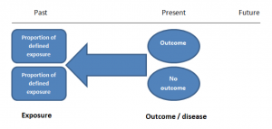
Figure 1. Case-control study design.

Cases should be selected based on objective inclusion and exclusion criteria from a reliable source such as a disease registry. An inherent issue with selecting cases is that a certain proportion of those with the disease would not have a formal diagnosis, may not present for medical care, may be misdiagnosed or may have died before getting a diagnosis. Regardless of how the cases are selected, they should be representative of the broader disease population that you are investigating to ensure generalisability.

Case-control studies should include two groups that are identical EXCEPT for their outcome / disease status.

As such, controls should also be selected carefully. It is possible to match controls to the cases selected on the basis of various factors (e.g. age, sex) to ensure these do not confound the study results. It may even increase statistical power and study precision by choosing up to three or four controls per case (2).

Case-controls can provide fast results and they are cheaper to perform than most other studies. The fact that the analysis is retrospective, allows rare diseases or diseases with long latency periods to be investigated. Furthermore, you can assess multiple exposures to get a better understanding of possible risk factors for the defined outcome / disease.

Nevertheless, as case-controls are retrospective, they are more prone to bias. One of the main examples is recall bias. Often case-control studies require the participants to self-report their exposure to a certain factor. Recall bias is the systematic difference in how the two groups may recall past events e.g. in a study investigating stillbirth, a mother who experienced this may recall the possible contributing factors a lot more vividly than a mother who had a healthy birth.

A summary of the pros and cons of case-control studies are provided in Table 1.

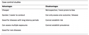
Table 1. Advantages and disadvantages of case-control studies.

Cohort studies

Cohort studies can be retrospective or prospective. Retrospective cohort studies are NOT the same as case-control studies.

In retrospective cohort studies, the exposure and outcomes have already happened. They are usually conducted on data that already exists (from prospective studies) and the exposures are defined before looking at the existing outcome data to see whether exposure to a risk factor is associated with a statistically significant difference in the outcome development rate.

Prospective cohort studies are more common. People are recruited into cohort studies regardless of their exposure or outcome status. This is one of their important strengths. People are often recruited because of their geographical area or occupation, for example, and researchers can then measure and analyse a range of exposures and outcomes.

The study then follows these participants for a defined period to assess the proportion that develop the outcome/disease of interest. See Figure 2 for a pictorial representation of a cohort study design. Therefore, cohort studies are good for assessing prognosis, risk factors and harm. The outcome measure in cohort studies is usually a risk ratio / relative risk (RR).

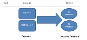
Figure 2. Cohort study design.

Cohort studies should include two groups that are identical EXCEPT for their exposure status.

As a result, both exposed and unexposed groups should be recruited from the same source population. Another important consideration is attrition. If a significant number of participants are not followed up (lost, death, dropped out) then this may impact the validity of the study. Not only does it decrease the study’s power, but there may be attrition bias – a significant difference between the groups of those that did not complete the study.

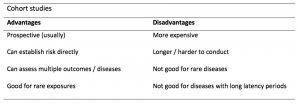
Cohort studies can assess a range of outcomes allowing an exposure to be rigorously assessed for its impact in developing disease. Additionally, they are good for rare exposures, e.g. contact with a chemical radiation blast.

Whilst cohort studies are useful, they can be expensive and time-consuming, especially if a long follow-up period is chosen or the disease itself is rare or has a long latency.

A summary of the pros and cons of cohort studies are provided in Table 2.

The Strengthening of Reporting of Observational Studies in Epidemiology Statement (STROBE)

STROBE provides a checklist of important steps for conducting these types of studies, as well as acting as best-practice reporting guidelines (3). Both case-control and cohort studies are observational, with varying advantages and disadvantages. However, the most important factor to the quality of evidence these studies provide, is their methodological quality.

• Song, J. and Chung, K. Observational Studies: Cohort and Case-Control Studies .  Plastic and Reconstructive Surgery.  2010 Dec;126(6):2234-2242.
• Ury HK. Efficiency of case-control studies with multiple controls per case: Continuous or dichotomous data .  Biometrics . 1975 Sep;31(3):643–649.
• von Elm E, Altman DG, Egger M, Pocock SJ, Gøtzsche PC, Vandenbroucke JP; STROBE Initiative.  The Strengthening the Reporting of Observational Studies in Epidemiology (STROBE) statement: guidelines for reporting observational studies.   Lancet 2007 Oct;370(9596):1453-14577. PMID: 18064739.

Saul Crandon

Leave a reply cancel reply.

Your email address will not be published. Required fields are marked *

Save my name, email, and website in this browser for the next time I comment.

No Comments on Case-control and Cohort studies: A brief overview

Very well presented, excellent clarifications. Has put me right back into class, literally!

Very clear and informative! Thank you.

very informative article.

Thank you for the easy to understand blog in cohort studies. I want to follow a group of people with and without a disease to see what health outcomes occurs to them in future such as hospitalisations, diagnoses, procedures etc, as I have many health outcomes to consider, my questions is how to make sure these outcomes has not occurred before the “exposure disease”. As, in cohort studies we are looking at incidence (new) cases, so if an outcome have occurred before the exposure, I can leave them out of the analysis. But because I am not looking at a single outcome which can be checked easily and if happened before exposure can be left out. I have EHR data, so all the exposure and outcome have occurred. my aim is to check the rates of different health outcomes between the exposed)dementia) and unexposed(non-dementia) individuals.

Very helpful information

Thanks for making this subject student friendly and easier to understand. A great help.

Thanks a lot. It really helped me to understand the topic. I am taking epidemiology class this winter, and your paper really saved me.

Happy new year.

Wow its amazing n simple way of briefing ,which i was enjoyed to learn this.its very easy n quick to pick ideas .. Thanks n stay connected

Saul you absolute melt! Really good work man

am a student of public health. This information is simple and well presented to the point. Thank you so much.

very helpful information provided here

really thanks for wonderful information because i doing my bachelor degree research by survival model

Quite informative thank you so much for the info please continue posting. An mph student with Africa university Zimbabwe.

Thank you this was so helpful amazing

Apreciated the information provided above.

So clear and perfect. The language is simple and superb.I am recommending this to all budding epidemiology students. Thanks a lot.

Great to hear, thank you AJ!

I have recently completed an investigational study where evidence of phlebitis was determined in a control cohort by data mining from electronic medical records. We then introduced an intervention in an attempt to reduce incidence of phlebitis in a second cohort. Again, results were determined by data mining. This was an expedited study, so there subjects were enrolled in a specific cohort based on date(s) of the drug infused. How do I define this study? Thanks so much.

thanks for the information and knowledge about observational studies. am a masters student in public health/epidemilogy of the faculty of medicines and pharmaceutical sciences , University of Dschang. this information is very explicit and straight to the point

Very much helpful

Subscribe to our newsletter

You will receive our monthly newsletter and free access to Trip Premium.

Related Articles

Cluster Randomized Trials: Concepts

This blog summarizes the concepts of cluster randomization, and the logistical and statistical considerations while designing a cluster randomized controlled trial.

Expertise-based Randomized Controlled Trials

This blog summarizes the concepts of Expertise-based randomized controlled trials with a focus on the advantages and challenges associated with this type of study.

An introduction to different types of study design

Conducting successful research requires choosing the appropriate study design. This article describes the most common types of designs conducted by researchers.

Study Design 101: Case Control Study

• Case Report
• Case Control Study
• Cohort Study
• Randomized Controlled Trial
• Practice Guideline
• Systematic Review
• Meta-Analysis
• Helpful Formulas
• Finding Specific Study Types

A study that compares patients who have a disease or outcome of interest (cases) with patients who do not have the disease or outcome (controls), and looks back retrospectively to compare how frequently the exposure to a risk factor is present in each group to determine the relationship between the risk factor and the disease.

Case control studies are observational because no intervention is attempted and no attempt is made to alter the course of the disease. The goal is to retrospectively determine the exposure to the risk factor of interest from each of the two groups of individuals: cases and controls. These studies are designed to estimate odds.

Case control studies are also known as "retrospective studies" and "case-referent studies."

• Good for studying rare conditions or diseases
• Less time needed to conduct the study because the condition or disease has already occurred
• Lets you simultaneously look at multiple risk factors
• Useful as initial studies to establish an association
• Can answer questions that could not be answered through other study designs

Disadvantages

• Retrospective studies have more problems with data quality because they rely on memory and people with a condition will be more motivated to recall risk factors (also called recall bias).
• Not good for evaluating diagnostic tests because it's already clear that the cases have the condition and the controls do not
• It can be difficult to find a suitable control group

Design pitfalls to look out for

Care should be taken to avoid confounding, which arises when an exposure and an outcome are both strongly associated with a third variable. Controls should be subjects who might have been cases in the study but are selected independent of the exposure. Cases and controls should also not be "over-matched."

Is the control group appropriate for the population? Does the study use matching or pairing appropriately to avoid the effects of a confounding variable? Does it use appropriate inclusion and exclusion criteria?

Fictitious Example

There is a suspicion that zinc oxide, the white non-absorbent sunscreen traditionally worn by lifeguards is more effective at preventing sunburns that lead to skin cancer than absorbent sunscreen lotions. A case-control study was conducted to investigate if exposure to zinc oxide is a more effective skin cancer prevention measure. The study involved comparing a group of former lifeguards that had developed cancer on their cheeks and noses (cases) to a group of lifeguards without this type of cancer (controls) and assess their prior exposure to zinc oxide or absorbent sunscreen lotions.

This study would be retrospective in that the former lifeguards would be asked to recall which type of sunscreen they used on their face and approximately how often. This could be either a matched or unmatched study, but efforts would need to be made to ensure that the former lifeguards are of the same average age, and lifeguarded for a similar number of seasons and amount of time per season.

Real-life Examples

Boubekri, M., Cheung, I., Reid, K., Wang, C., & Zee, P. (2014). Impact of windows and daylight exposure on overall health and sleep quality of office workers: a case-control pilot study. Journal of Clinical Sleep Medicine : JCSM : Official Publication of the American Academy of Sleep Medicine, 10 (6), 603-611. https://doi.org/10.5664/jcsm.3780

This pilot study explored the impact of exposure to daylight on the health of office workers (measuring well-being and sleep quality subjectively, and light exposure, activity level and sleep-wake patterns via actigraphy). Individuals with windows in their workplaces had more light exposure, longer sleep duration, and more physical activity. They also reported a better scores in the areas of vitality and role limitations due to physical problems, better sleep quality and less sleep disturbances.

Togha, M., Razeghi Jahromi, S., Ghorbani, Z., Martami, F., & Seifishahpar, M. (2018). Serum Vitamin D Status in a Group of Migraine Patients Compared With Healthy Controls: A Case-Control Study. Headache, 58 (10), 1530-1540. https://doi.org/10.1111/head.13423

This case-control study compared serum vitamin D levels in individuals who experience migraine headaches with their matched controls. Studied over a period of thirty days, individuals with higher levels of serum Vitamin D was associated with lower odds of migraine headache.

Related Formulas

• Odds ratio in an unmatched study
• Odds ratio in a matched study

Related Terms

A patient with the disease or outcome of interest.

Confounding

When an exposure and an outcome are both strongly associated with a third variable.

A patient who does not have the disease or outcome.

Matched Design

Each case is matched individually with a control according to certain characteristics such as age and gender. It is important to remember that the concordant pairs (pairs in which the case and control are either both exposed or both not exposed) tell us nothing about the risk of exposure separately for cases or controls.

Observed Assignment

The method of assignment of individuals to study and control groups in observational studies when the investigator does not intervene to perform the assignment.

Unmatched Design

The controls are a sample from a suitable non-affected population.

Now test yourself!

1. Case Control Studies are prospective in that they follow the cases and controls over time and observe what occurs.

a) True b) False

2. Which of the following is an advantage of Case Control Studies?

a) They can simultaneously look at multiple risk factors. b) They are useful to initially establish an association between a risk factor and a disease or outcome. c) They take less time to complete because the condition or disease has already occurred. d) b and c only e) a, b, and c

Evidence Pyramid - Navigation

• Meta- Analysis
• Case Reports
• << Previous: Case Report
• Next: Cohort Study >>

• Last Updated: Sep 25, 2023 10:59 AM
• URL: https://guides.himmelfarb.gwu.edu/studydesign101

• Himmelfarb Intranet
• Privacy Notice
• Terms of Use
• GW is committed to digital accessibility. If you experience a barrier that affects your ability to access content on this page, let us know via the Accessibility Feedback Form .
• Himmelfarb Health Sciences Library
• 2300 Eye St., NW, Washington, DC 20037
• Phone: (202) 994-2850
• [email protected]
• https://himmelfarb.gwu.edu

Case-control studies: advantages and disadvantages

Affiliation.

• 1 Centre for Medical and Healthcare Education, St George's, University of London, London, UK [email protected].
• PMID: 31419845
• DOI: 10.1136/bmj.f7707

Case-Control Studies

Chris nickson.

• Nov 3, 2020
• a type of retrospective observational study
• control patients are ‘matched’ using some criteria (age, gender), typically should have no history of the disease of interest and should be representative of the general population
• begins with a definition of outcome or interest
• aims to identify potential risk factors associated with outcomes
• measures exposure to risk factors
• outcome = in case and controls
• odds ratio used to quantify risk, and can be adjusted for confounders (e.g. using logistic regression)
• quick, cheap and easy
• cases and controls may be sampled from pre-existing databases
• useful for identifying possible risk factors of a condition
• useful for studying rare conditions and those with a long latency period following exposure to risk
• not prone to loss to follow-up, unlike cohort studies
• may be used as the initial study generating hypotheses to be studied further by larger, more expensive prospective studies

DISADVANTAGES

• controls are often recruited by convenience sampling, and are thus not representative of the general population and prone to selection bias
• subject to confounding (other risk factors may be present that were not measured)
• not always possible in case-control studies to predict whether exposure to the risk factors preceded development of the disease or condition
• relative risk can not be determined as the incidence or prevalence of the condition of interest cannot be estimated in the population
• not suitable if exposure to the risk factors of interest is rare, as few of the cases and controls will have been exposed to them
• cannot determine causation, only association

Critical Care

Chris is an Intensivist and ECMO specialist at the  Alfred ICU in Melbourne. He is also a Clinical Adjunct Associate Professor at Monash University . He is a co-founder of the  Australia and New Zealand Clinician Educator Network  (ANZCEN) and is the Lead for the  ANZCEN Clinician Educator Incubator  programme. He is on the Board of Directors for the  Intensive Care Foundation  and is a First Part Examiner for the  College of Intensive Care Medicine . He is an internationally recognised Clinician Educator with a passion for helping clinicians learn and for improving the clinical performance of individuals and collectives.

After finishing his medical degree at the University of Auckland, he continued post-graduate training in New Zealand as well as Australia’s Northern Territory, Perth and Melbourne. He has completed fellowship training in both intensive care medicine and emergency medicine, as well as post-graduate training in biochemistry, clinical toxicology, clinical epidemiology, and health professional education.

He is actively involved in in using translational simulation to improve patient care and the design of processes and systems at Alfred Health. He coordinates the Alfred ICU’s education and simulation programmes and runs the unit’s education website,  INTENSIVE .  He created the ‘Critically Ill Airway’ course and teaches on numerous courses around the world. He is one of the founders of the  FOAM  movement (Free Open-Access Medical education) and is co-creator of  litfl.com , the  RAGE podcast , the  Resuscitology  course, and the  SMACC  conference.

His one great achievement is being the father of three amazing children.

On Twitter, he is  @precordialthump .

| INTENSIVE | RAGE | Resuscitology | SMACC

Leave a Reply Cancel reply

This site uses Akismet to reduce spam. Learn how your comment data is processed .

Privacy Overview

An official website of the United States government

The .gov means it’s official. Federal government websites often end in .gov or .mil. Before sharing sensitive information, make sure you’re on a federal government site.

The site is secure. The https:// ensures that you are connecting to the official website and that any information you provide is encrypted and transmitted securely.

• Publications
• Account settings

Preview improvements coming to the PMC website in October 2024. Learn More or Try it out now .

• Advanced Search
• Journal List
• Int J Biostat

Why Match? Investigating Matched Case-Control Study Designs with Causal Effect Estimation *

Sherri rose.

* University of California, Berkeley, ude.yelekreb@irrehs

Mark J. van der Laan

† University of California, Berkeley, ude.yelekreb@naal

Matched case-control study designs are commonly implemented in the field of public health. While matching is intended to eliminate confounding, the main potential benefit of matching in case-control studies is a gain in efficiency. Methods for analyzing matched case-control studies have focused on utilizing conditional logistic regression models that provide conditional and not causal estimates of the odds ratio. This article investigates the use of case-control weighted targeted maximum likelihood estimation to obtain marginal causal effects in matched case-control study designs. We compare the use of case-control weighted targeted maximum likelihood estimation in matched and unmatched designs in an effort to explore which design yields the most information about the marginal causal effect. The procedures require knowledge of certain prevalence probabilities and were previously described by van der Laan (2008) . In many practical situations where a causal effect is the parameter of interest, researchers may be better served using an unmatched design.

1. Introduction

Individually matched case-control study designs are frequently found in public health and medical literature, and conditional logistic regression is the tool most commonly used to analyze these studies. Matching is intended to eliminate confounding, however, the main potential benefit of matching in case-control studies is a gain in efficiency. Therefore, when are these study designs truly beneficial? Given all the potential drawbacks, including extra cost, added time for enrollment, and increased bias, the use of matching in case-control study designs warrants careful evaluation. Discussion of the advantages and disadvantages of matching in the literature goes back more than 40 years.

In this paper, we focus on individual matching in case-control studies where the researcher is interested in estimating the marginal causal effect, and certain prevalence probabilities are known. Our procedure, first presented in van der Laan (2008) , “targets” the parameter of interest rather than the distribution of interest, and is thus aptly named case-control weighted targeted maximum likelihood estimation. In order to eliminate the bias caused by the matched case-control sampling design, this technique relies on knowledge of the true prevalence probability q 0 ≡ P 0 * ( Y = 1 ) , and an additional value q ¯ 0 ( M ) ≡ q 0 P 0 * ( Y = 0 | M ) P 0 * ( Y = 1 | M ) , where M is the matching variable. For unmatched designs, knowledge of only q 0 is required.

The case-control weighting scheme maps estimation methods developed for prospective sampling into methods for case-control sampling, and it produces efficient estimators when its prospective sample counterpart is efficient. Thus, both the matched and unmatched procedures are double robust and locally efficient: they perform well as long as P 0 * ( Y | A ,   W ) or P 0 * ( A | W ) is correctly specified, are consistent if either of these models are correctly specified, and efficient if both are correctly specified. (Here A is the exposure of interest and If is a vector of covariates.) We will compare the use of case-control weighted targeted maximum likelihood estimation in matched and unmatched case-control study designs as we explore which design yields the most information about the marginal causal effect. This paper will not address matching in cohort studies, and will concentrate solely on case-control studies. However, matching in cohort studies was briefly addressed in van der Laan (2008) , and applying our methods to cohort studies is an area of future research.

2. Why Match? A Literature Review

There is a large collection of literature devoted to the topic of individual matching in case-control study designs. This overview attempts to capture the most important consideratons, and it is by no means exhaustive.

2.1. Individual Matching in Case-Control Studies

In an individually matched case-control study, the population of interest is identified, and cases are randomly sampled or selected based on particular inclusion criteria. Although, as Rothman and Greenland (1998) note, the definition of a case may implicitly define the population of interest for cases and controls. Each of these cases is then matched to one or more controls based on a variable (or variables) believed to be a confounder. Much of the literature on individual matching in case-control studies, particularly earlier texts, describes these designs as a way to reduce confounding in the sampling design. Reference to this is made in: Miettinen (1970) , Breslow et al. (1978) , Breslow and Day (1980) , Kupper et al. (1981) , Schlesselman (1982) , Collett (1991) , and Costanza (1995) , among others. However, several authors ( Breslow and Day, 1980 ; Kupper et al., 1981 ; Schlesselman, 1982 ; Rothman and Greenland, 1998 ; Vandenbroucke et al., 2007 ) point out that the goal of matching is to increase the study’s efficiency by forcing the case and control samples to have similar distributions across confounding variables. Rothman and Greenland (1998) go on to say that while matching is intended to control confounding, it cannot do this in case-control study designs, and can, in fact, introduce bias. Costanza (1995) agreed, stating that matching on confounders in case-control studies does nothing to remove the confounding, but frequently introduces negative confounding.

So, while some literature cites the purpose of matching as improving validity, later publications ( Kupper et al., 1981 ; Rothman and Greenland, 1998 ) demonstrated that matching has a greater impact on efficiency over validity. Matched sampling leads to a balanced number of cases and controls across the levels of the selected matching variables. This balance can reduce the variance in the parameters of interest, which improves statistical efficiency. A study with a randomly selected control group may yield some strata with an imbalance of cases and controls. It is important to add, however, that matching in case-control studies can lead to gains or losses in efficiency ( Kupper et al., 1981 ; Rothman and Greenland, 1998 ). This will be discussed further in later sections.

Breslow and Day (1980) note that matched case-control studies attempt to increase the informativeness of each of the subjects in the study. However, one should also note that matched studies discard not only a pool of unmatched controls, but the information in each exposure-concordant case-control pair. Additionally, matching has a substantial impact on the study sample, most notably, it creates a sample of controls that is not representative of exposure in the population or the population as a whole. The effect of the matching variable can no longer be studied directly, and the exposure frequency in the control sample will be shifted towards that of the cases ( Rothman and Greenland, 1998 ). Matching in case-control studies also does not completely control for the variable or variables used for matching, in general. This means that researchers who implement matched designs must perform matched or stratified analyses ( Seigel and Greenhouse, 1973 ; Schlesselman, 1982 ; Holland and Rubin, 1988 ; Rothman and Greenland, 1998 ; Rubin, 2006 ). If an unmatched analysis is performed on matched data, the validity of the case-control comparison may be decreased ( Schlesselman, 1982 ).

2.2. Variable Selection

We revisit an earlier point made in this overview of individually matched case-control studies: matching variables are chosen a priori on the belief that they confound the relationship between exposure and disease. If controls are matched to cases based on a variable that is not a true confounder, this can impact efficiency. For example, if the matching variable is not associated with disease but is associated with the exposure, this will increase the variance of the estimator compared to an unmatched design. Here, the matching leads to larger numbers of exposure-concordant case-control pairs, which are not informative in the analysis, leading to the increase in variance. If the matching variable is only associated with disease, there is often a loss of efficiency as well ( Schlesselman, 1982 ). If the matching variable is along the causal pathway between disease and exposure then matching will contribute bias that cannot be removed in the analysis ( Vandenbroucke et al., 2007 ). Matching on a variable associated with exposure and not disease or a variable along the causal pathway are considered types of overmatching . Variables for matching should therefore be selected very carefully, and only those that are known to be associated with both exposure and disease should be considered. The number of matching variables should also be reduced to as few as possible. As the number of matching variables grows, the cases and controls will become increasingly similar with respect to the exposure of interest, and the study may produce a spurious result or provide no information ( Breslow and Day, 1980 ). Additionally, when matching on more than one variable, matching variables should not be strongly correlated with each other ( Schlesselman, 1982 ).

2.3. More on Efficiency

Kupper et al. (1981) performed a variety of simulations to demonstrate the impact of matching on efficiency. They found that in situations where confounding was present, the confidence intervals for matched studies were smaller than unmatched studies unless the odds ratio and the exposure of interest were large. However, the confidence intervals for the samples with randomly selected controls were always shorter when the number of controls was at least twice that of the cases. This is an important result, as efficiency is often touted as the benefit of an individually matched case-control study design. Simulations aside, Cochran (1953) is often cited as the theoretical paper that demonstrates the efficiency of matched designs. However, as noted by McKinlay (1977) , Cochran’s result can be misleading. Comparisons between matched and unmatched study designs are often made with equal sample sizes and no other method of covariate adjustment (e.g. regression). In a matched design, controls may be discarded if they do not match a particular case on the variable or variables of interest. Multiple controls may be discarded per case, depending on the variables of interest ( Freedman, 1950 ; Cochran and Chambers, 1965 ; McKinlay, 1977 ). In a typical randomly selected case-control study, these controls would be included. In many cases, if the discarded controls were available to be rejected in the matched study, they would be available for an unmatched design in the same investigation ( Billewicz, 1965 ; McKinlay, 1977 ). Therefore, it may be more appropriate to compare the efficiencies of matched case-control studies of size n to randomly selected case-control studies of size n+number of discarded controls . Additionally, these randomly selected case-control studies should employ a method of analysis to reduce bias and variance. Therefore, the result from Kupper et al. (1981) is especially poignant, as all randomly selected case-control studies that had a size of at least 2n had shorter confidence intervals than their matched counterparts of size n .

2.4. Trends

Gefeller et al. (1998) performed a literature review of case-control studies published between 1955 and 1994 in three main epidemiology journals: American Journal of Epidemiology, International Journal of Epidemiology, and the Journal of Epidemiology and Community Health . They found that, among these journals, there was a decreasing trend in the percentage of individually matched case-control studies published (71.7% in the years preceding 1981, 65.5% in 1985, 46.9% in 1989, and 46.4% in 1994), and an increasing percentage of frequency matched studies (5.0% in the years preceding 1981, 9.1% in 1985, 16.3% in 1989, and 26.2% in 1994). Interestingly, the percentage of case-control studies using no matching stayed relatively constant with no obvious trend (averaging 29.3%, and ranging from 23.2% to 36.7%). Unfortunately, they found substantial evidence that individually matched studies were being performed without the appropriate matched analysis: only 74% of studies from 1994 used conditional logistic regression if logistic regression was the chosen method of analysis. A later analysis of medical literature in Medline, Rahman (2003) , indicated that 5.3% of individually matched case-control studies used an unconditional logistic regression for those selecting logistic regression models. The review in Gefeller et al. (1998) indicates that unmatched case-control studies, at least in epidemiology, are in the minority. This should be questioned given the overwhelming agreement in the literature that matching is not frequently justified for case-control study designs.

2.5. Literature Review Discussion

The consensus in the literature indicates that there are very few circumstances where individual matching is indeed warranted. Case-control studies with a very small number of cases may benefit from individual matching, as a randomly selected control group from even a well-defined population of interest may be uninformative on many variables of interest ( Schlesselman, 1982 ; Costanza, 1995 ). Individual matching moves from beneficial to required when variables such as sibship are included in the study ( Rothman and Greenland, 1998 ; Costanza, 1995 ). Matching is also cited as necessary by many authors when the investigators expect the distribution of the matching variable to differ drastically between the cases and the controls. It may be this reason that draws many investigators towards a matched design, perhaps without appropriate consideration of the disadvantages or definition of the population of interest.

Methodologists in the literature stress that it is often possible for confounders to be adjusted for in the analysis instead of matched on in case-control designs ( Schlesselman, 1982 ; Vandenbroucke et al., 2007 ). The development of effective methods to control confounding in analyses may have contributed to the drop in individually matched designs, but they are still quite common. It is therefore important to continue to disseminate the implications of individually matched case-control study designs to researchers, as Rothman and Greenland (1998) note that “people match on a variable (e.g. sex) simply because it is the ‘expected thing to do’ and they might lose credibility for not matching.” When researchers make design and analysis decisions based on these types of considerations, their research may suffer.

Our contributions to the vast literature on individual matching for case-control studies will be unique. We focus on scenarios where the researcher is interested in estimating a marginal causal effect, a parameter that cannot be estimated with conditional logistic regression, and certain prevalence probabilities are known. Thus, we will compare the use of case-control weighted targeted maximum likelihood estimation in matched and unmatched designs in an effort to explore which design yields the most information about the marginal causal effect.

3. Existing Methods

Model-based methods for the analysis of matched case-control studies are plentiful in recent literature ( Breslow et al., 1978 ; Holford et al., 1978 ; Breslow and Day, 1980 ; Greenland, 1981 ; Schlesselman, 1982 ; Holland and Rubin, 1988 ; Benichou and Wacholder, 1994 ; Rothman and Greenland, 1998 ; Greenland, 2004 ). And, while it is not the only method of analysis for individually matched case-control studies, the predominant method of analysis is conditional logistic regression. This method provides a conditional estimate of the odds ratio of being diseased given the exposure of interest and baseline covariates. Conditional logistic regression will be discussed in more detail in the subsection below. Greenland (1981) and Holland and Rubin (1988) discuss another model-based method: the use of log-linear models to estimate the marginal odds ratio. Additionally, Rothman and Greenland (1998) and Greenland (2004) demonstrate the use of standardization in case-control studies, which estimate marginal effects with population or person-time averaging. Holland and Rubin (1988) note that the traditional two-way table and its extensions generally provide no causal insight for matched case-control studies. However, these methods are all distinctly different from the method we illustrate in this paper, discussed by van der Laan (2008) , as our method is a nonparametric double robust locally efficient procedure that provides an estimate of the marginal causal odds ratio.

3.1. Conditional Logistic Regression

The logistic regression model for matched case-control studies differs from unmatched studies in that it allows the intercept to vary among the matched units of cases and controls. The matching variable is not included in the model ( Breslow et al., 1978 ; Holford et al., 1978 ; Breslow and Day, 1980 ; Schlesselman, 1982 ). If the parameter of interest is the coefficient in front of the exposure A, the use of a matched study design and a conditional logistic regression analysis can yield increases in efficiency, compared to an unmatched design with a logistic regression analysis. It is important to note that in order to estimate an effect of exposure A with conditional logistic regression, the case and control must be discordant on A . Additionally, if information for a variable is missing; for a case (or control), the corresponding control (or case) information is discarded ( Breslow and Day, 1980 ; Schlesselman, 1982 ). These two limitations do not occur in the new case-control weighted targeted maximum likelihood estimation methodology for causal effect parameters. More importantly, if a marginal causal effect is the parameter of interest, conditional logistic regression cannot be used as it can only estimate the conditional odds ratio.

4. Case-Control Weighted Targeted Maximum Likelihood Estimation

4.1. background.

We define O * = ( W , A , Y )   ∼   P 0 * as the experimental unit and corresponding distribution P 0 * of interest. P 0 * represents the population from which all cases and controls will be sampled. Here O* consists of baseline covariates W, an exposure variable A (referred to as the “treatment” variable in prospective studies), and a binary outcome Y, which defines case or control status. If we are interested in marginal causal effect parameters, we can define ψ 0 * = Ψ * ( P 0 * ) ∈ IR d of P 0 * ∈ M * as the causal effect parameter and define the risk difference, relative risk, odds ratio as follows for binary exposure A ∈ {0, 1}:

These causal versions of the effect parameters require the specification of the counterfactual outcomes Y 0 and Y 1 for binary A and ( W , A, Y = Y A ) as a time-ordered missing data structure on the full data structure ( W , Y 0 , Y 1 ). One must also make the randomization assumption: { A ⊥ Y 0 , Y 1 | W }. Since these parameters are always well defined parameters of the distribution of the data, they can thereby be viewed as W -adjusted variable importance parameters. Then there is no need to make these assumptions. We refer to van der Laan (2006) for the details of this framework.

However, the observed data structure in matched case-control sampling is defined by:

Here M ⊂ W, and M is a categorical matching variable. The sampling distribution of the data structure O is described as above with P 0 . Thus, the matched case-control data set contains n independent and identically distributed observations O 1 ,..., O n with sampling distribution P 0 . The cluster containing one case and the J controls is the experimental unit, and the marginal distribution of the cluster is specified by the population distribution P 0 * . The model M * , which possibly includes knowledge of q 0 or q ̄ 0 ( M ), then implies models for the marginal distribution of cases ( M 1 , W 1 , A 1 ) and controls ( M 1 ,   W 2 j ,   A 2 j ) , j = 1,..., J .

Independent case-control sampling is described as sampling nC cases from the conditional distribution of ( W , A ), given Y = 1, and sampling nCo controls from ( W, A ), given Y = 0. The value of J used to weight each control is then nCo/nC . We refer to independent case-control sampling as Case-Control Design I, and matched case-control sampling as Case-Control Design II.

4.2. Methodology Summary

If one wishes to estimate marginal causal effects for Case-Control Design II, which correspond with the traditional parameters of interest in randomized trials, there is now a nonparametric double robust locally efficient procedure available. It performs well as long as P 0 * ( Y | A ,     W ) or P 0 * ( A | W ) is correctly specified, is consistent if either of these models are correctly specified, and efficient if both are correctly specified. The theoretical framework for case-control weighted targeted maximum likelihood estimation has been discussed in detail in van der Laan (2008) , and step-by-step implementation for Case-Control Design I appears in Rose and van der Laan (2008) . For the targeted maximum likelihood framework designed for prospective sampling, see van der Laan (2006) , and for its implementation, see Bembom et al. (2007) .

Case-control weighted targeted maximum likelihood estimation for Case-Control Design II incorporates estimates of P 0 * ( Y | A ,     W ) , P 0 * ( A | W ) , and knowledge of q 0 and q ̄ 0 ( M ), where q ̄ 0 (M) is defined as:

The case-control weighted targeted maximum likelihood estimation procedure for Case-Control Design II uses P 0 * ( A | W ) to update an initial estimate of P 0 * ( Y | A ,     W ) .

4.3. Implementation

Case-control weighted targeted maximum likelihood estimation for Case-Control Designs I and II can be implemented using existing software (including SAS, STATA, and R). The implementation of case-control weighted targeted maximum likelihood for Case-Control Design II is also very similar to the implementation for Case-Control Design I. Key differences will be stressed here, but for more detail, we refer to Rose and van der Laan (2008) .

Weights q 0 and q ¯ 0 ( M ) 1 J are assigned to the cases and corresponding J controls, respectively. This differs from Case-Control Design I in that ( 1 − q 0 ) 1 J is used to weight controls in Case Control Design I instead of q ¯ 0 ( M ) 1 J . In van der Laan (2008) it is suggested that in cases where q ̄ 0 ( M ) is not known, 1 – q 0 can be used to approximate q ̄ 0 ( M ).

Estimating Q 0 * ( A ,     W )

Estimate P 0 * ( Y | A ,   W ) ≡ Q 0 * ( A ,   W ) using the appropriate weights. This estimate is denoted Q ̂ *(A, W) . Two methods for estimating Q ̂ *(A, W) include intercept adjusted logistic regression and case-control weighted logistic regression. Intercept adjusted logistic regression adds the intercept log q 0 /( 1 – q 0 ) to a logistic regression model. This yields the true logistic regression function P 0 * ( Y = 1 | A ,     W ) . If intercept adjusted logistic regression is used to obtain Q ̂ *(A, W), cases are weighted 1 and controls are weighted with q ¯ 0 ( M ) 1 J . This is the only step and method where assigned weights are not q 0 and q ¯ 0 ( M ) 1 J . In Rose and van der Laan (2008) , we discussed disadvantages associated with using intercept adjusted logistic regression, and thus our simulations will focus on the use of case-control weighted logistic regression for estimating Q 0 * ( A ,     W ) .

Case-control weighted logistic regression uses the assigned weights and performs maximum likelihood estimation for prospective sampling (ignoring the case-control sampling design). Consider a nonparametric model for the marginal distribution of the covariates, and a model { Q θ * : θ } for Q 0 * ( A ,     W ) . Then the case-control weighted maximum likelihood estimator for Q 0 * ( A ,     W ) in Case-Control Design II is given by:

If Q ̂ *(A, W) is obtained using case-control weighted logistic regression, it is weighted with q 0 and q ¯ 0 ( M ) 1 J . For further discussion see van der Laan (2008) and Rose and van der Laan (2008) .

Estimating g 0 * ( A | W )

Estimate P 0 * ( A | W ) ≡ g 0 * ( A + W ) using assigned weights. This estimate is denoted ĝ*(A | W), and may be obtained using case-control weighted logisitic regression, for example.

Calculating h(A, W)

Calculate the “clever covariate” for each subject based on g 0 * ( A | W ) . The covariate takes the form:

for the risk difference. Two covariates are used for estimation of other parameters, such as the odds ratio:

For further discussion see van der Laan and Rubin (2006) and Moore and van der Laan (2007) .

Updating Q ̂ * (A, W)

Update Q ̂ * (A , W) by performing an additional weighted regression with h(A, W) as a supplementary covariate. The other coefficients in the initial fit Q ̂ *(A, W) are held fixed, and the intercept is suppressed in order to estimate the case-control weighted estimator of ε, the coefficient in front of h(A, W), which we denote as ɛ̂ 1 . The regression estimate Q ̂ *(A, W) is then updated and given by Q ^ 1 * ( A ,     W ) :

This step is iterated until convergence, although convergence is often achieved in one step.

Estimating Causal Parameters

Using q 0 , q ̄ 0 (M 1 ), and Q ^ 1 * ( A ,     W ) , estimate causal parameters of interest (risk difference, relative risk, and odds ratio, defined in formulas (1), (2), and (3)) by averaging over the case-control weighted distribution of W . This mapping is performed by evaluating Q ^ 1 * ( A ,     W ) at A = 1 and A = 0 and applying weights q 0 to cases and q ¯ 0 ( M 1 ) 1 J to the controls. This forms case-control weighted estimates of E 0 * ( Y 1 ) = P 0 * ( Y 1 = 1 ) and E 0 * ( Y 0 ) = P 0 * ( Y 0 = 1 ) . The causal parameters of interest can then be calculated from these estimates. For example, the relative risk E 0 * ( Y 1 ) / E 0 * ( Y 0 ) is estimated by:

Calculating Standard Errors

Calculating standard errors, p-values, and confidence intervals for case-control weighted targeted maximum likelihood estimates requires the use of the case-control weighted influence curve. This methodology is discussed in detail in van der Laan (2008) . We also refer to van der Laan and Robins (2002) for careful discussions of gradients and influence curve theory. The case-control weighted influence curve for matched case-control study designs is the influence curve for prospective targeted maximum likelihood with case-control weighting. We refer to van der Laan and Rubin (2006) and Moore and van der Laan (2007) for this methodology. A complete understanding of the derivation of infuence curves is not required to implement the case-control targeted maximum likelihood estimation procedure for Case-Control Design II.

For illustration, we present the unweighted influence curve for the risk difference of a prospective study ψ 0 , R D * = P 0 * ( Y 1 = 1 ) − P 0 * ( Y 0 = 1 ) , which is estimated by:

The case-control weighted double robust efficient influence curve for the risk difference ψ 0 , R D * = P 0 * ( Y 1 = 1 ) − P 0 * ( Y 0 = 1 ) in a matched case-control study design is then:

The asymptotic variance of n ( ψ ^ − ψ 0 * ) using the estimate of the efficient influence curve D q 0 (ψ* , g* , Q *)( O ) can be estimated by:

A 95% Wald-type confidence interval can then be constructed using the causal parameter estimate ψ ^ : ψ ^ ± z 0.975 σ ^ n , as well as a p-value for ψ ^ : 2 [ 1 − Φ ( | ψ ^ σ ^ / n | ) ] .

5. Simulation Studies

5.1. simulation 1.

Our first simulation study was designed to illustrate the differences between independent case-control sampling (Case-Control Design I) and matched case-control sampling (Case-Control Design II) using the case-control weighting scheme for targeted maximum likelihood estimation proposed by van der Laan (2008) . It was also designed to represent “ideal” situations where control information is not discarded (e.g. data collection is expensive, and covariate information is only collected when a control is a match). This simulation also demonstrates the use of weights q 0 and ( 1 − q 0 ) 1 J with matched data, to represent situations where q ̄ 0 (M) is not known. The population contained N = 35, 000 individuals, where we simulated a 9-dimensional covariate W = (W i : i = 1,..., 9), a binary exposure (or “treatment”) A , and an indicator Y, which was 1 for cases and 0 for controls. These variables were generated according to the following rules:

It can be seen in both g 0 * ( A | W ) and Q 0 * ( A ,   W ) that the covariates were generated with varied levels of association with A and Y . This was done to investigate the role of weak, medium, and strong association between a matching variable W i and A and Y . The corresponding associations can be seen in Figure 1 . For example, W 1 was weakly associated with both A and Y . One might recall that matching is potentially beneficial only when the matching variable is a true confounder; associated with both A and Y .

Simulated Covariates

Another illustration of the varied association levels can be seen in Figure 2 . Here, we display the probability an individual in the population was a case given W i = 1, all the non-matching covariates ( Z ), and A . Likewise, probabilities for W i = 0 are also shown. For example, let’s say matching variable W 2 is age with 1 representing ‘young’ (< 50 years) and 0 representing ‘old’ (≥ 50 years). In this population, it was not very likely (0.013) that someone who is young will become a case, while someone who is old has a much higher chance of becoming a case (0.047), given Z and A . Therefore, W 2 , W 5 , and W 8 represent situations where the distribution of W i among cases and controls is very different. The covariates W 3 , W 6 , and W 9 represent situations where this difference is even more extreme.

Simulated Covariates: Probabilities. Z represents the remaining eight non-matching covariates.

The simulated population had a prevalence probability q 0 = 0.030, and exactly 1045 cases. The true value of the odds ratio was given by OR = 2.302, with P 0 * ( Y 1 = 1 ) = 0.055 and P 0 * ( Y 0 = 1 ) = 0.025 . We sampled the population using a varying number of cases nC = (200, 500, 1000) for both Case-Control Designs I and II, and for each sample size we ran 1000 simulations. For each simulation, the same sampled cases were used for Case Control Designs I and II. Controls were matched to cases on one variable (W i ) in Case-Control Design II for both 1:1 and 1:2 designs. The same number of controls were used in both Case-Control Designs I and II. Causal effect parameters were estimated using case-control weighted targeted maximum likelihood estimation (CCW T-MLE) for Case-Control Designs I and II with case-control weighted logistic regression for Q ̂ * (A, W) discussed in Section 4.3. The initial fit for the estimate of Q 0 * ( A ,     W ) was correctly specified as:

The initial fit for the exposure mechanism, which was the correct fit, was defined by:

Case-Control Designs I and II performed similarly with respect to bias for the nine covariates. When examining efficiency, there were consistent increases in efficiency when the association between W i and Y was high ( W 3 , W 6 , and W 9 ), when comparing Case-Control Design II to Case-Control Design I. Results when association with W i and Y was medium ( W 2 , W 5 , and W 8 ) were not entirely consistent, although covariates W 5 and W 8 did show increases in efficiency for Case-Control Design II for all or nearly all sample sizes. These results were in line with the consensus found in our literature search: that matching may produce gains in efficiency when the distribution of the matching variable differs drastically between the cases and the controls.

Simulation 1 also demonstrates the use of weights q 0 and ( 1 − q 0 ) 1 J with matched data, for situations where q ̄ 0 (M) is unknown for Case-Control Design II. This weighting scheme provided a reasonable approximation, yielding larger standard errors, but similar levels of bias for covariates with a weak association with Y . As association with Y increased, the estimate of the odds ratio became more biased. Mean squared errors and relative efficiencies for the odds ratio can be seen in Table 1 . Bias results can be seen in Figures 3 and ​ and4 4 .

Simulation 1 – Bias for 1:1 Matching. CCD I is CCW T-MLE for Case-Control Design I, CCD II is CCW T-MLE for Case-Control Design II with q ̄ 0 (M) weighting, and CCD II (w) is CCW T-MLE for Case-Control Design II with (1 – q 0 ) weighting.

Simulation 1 – Bias for 1:2 Matching. CCD I is CCW T-MLE for Case-Control Design I, CCD II is CCW T-MLE for Case-Control Design II with q ̄ 0 (M) weighting, and CCD II (w) is CCW T-MLE for Case-Control Design II with (1 – q 0 ) weighting.

II MSE is Mean Squared Error for Case-Control Design II with weights ( 1 − q 0 ) 1 J for CCW T-MLE, II RE is relative efficiency of Case-Control Design II CCW T-MLE with q ̄ 0 ( M) weights is relative efficiency of Case-Control Design I CCW T-MLE, all REs are in comparison to II MSE, and nC is Number of Cases.

5.2. Simulation 2

Our second simulation study was designed to address less ideal, and perhaps more common, situations where control information is discarded. Controls were sampled from the population of controls in Simulation 1 until a match on covariate W i was found for each case. Non-matches were returned to the population of controls. The number of total controls sampled to find sufficient matches was recorded for each simulation. This was the number of randomly sampled controls that was used for the corresponding Case-Control Design I simulation. The mean number of controls sampled to achieve 1:1 and 1:2 matching at each sample size is noted in Table 2 as nCo . For example, in order to obtain 200 controls matched on covariate W 1 in a 1:1 design, an average of 404 controls had to be sampled from the population. Thus, an average of 404 controls were used in the corresponding Case-Control Design I.

II MSE is Mean Squared Error for Case-Control Design II CCW T-MLE, I RE is Relative Efficiency of Case Control Design I CCW T-MLE Compared to Case-Control Design II MSE, nC is Number of Cases, nCo is Mean Number of Controls for Case-Control Design I.

Case-control weighted targeted maximum likelihood estimation was performed for Case-Control Designs I and II. Case-Control Design I outperformed Case-Control Design II with respect to efficiency and bias for all sample sizes and both 1:1 and 1:2 matching. This was not surprising given the mean number of controls in each of the control samples for Case-Control Design I (on average, about two times the number of controls in each control sample for Case-Control Design II). Additionally, as association between W i and Y increased, there was a trend that the number of controls necessary for complete matching also increased. A similar trend between A and W i was not apparent. When returning to the bias results, one can see that they do not vary greatly with association between W i and A or Y . Mean squared errors and relative efficiencies for the odds ratio can be seen in Table 2 . Bias results are displayed in Figure 5 .

Simulation 2 – Bias. CCD I is CCW T-MLE for Case-Control Design I and CCD II is CCW T-MLE for Case-Control Design II.

6. Discussion

The main benefit of a matched case-control study design is a potential increase in efficiency. However, an increase in efficiency is not automatic. If one decides to implement a matched case-control study design, matching variable selection is crucial. Numerous publications in our literature review indicated that matching on non-confounding variables is not beneficial, including Kupper et al. (1981) : “The futility of matching in [non-confounding situations] is clear...matching on [the variable] will have absolutely no effect on the distribution of the exposure variable in the diseased and nondiseased groups.” Therefore, increases in efficiency with a matched design depend heavily on the selection of a confounding variable as a matching variable. In practice, it may be difficult to ascertain the strength of the association between the matching variable, the exposure of interest, and the outcome. Our simulations for causal effect estimation confirmed the consensus in the existing literature: that in situations where the distribution of the matching covariate is drastically different between the case and control populations, matching may provide an increase in efficiency. Our simulations indicated that P 0 * ( Y = 1 | W i = 1 ,     Z ,     A ) , for matching variable W i and covariate vector Z , may need to be very small for an increase in efficiency using a matched design. These results were true, however, only for our simulations where no control subjects were discarded] it is very common for matched study designs to discard controls ( Freedman, 1950 ; Cochran and Chambers, 1965 ; Billewicz, 1965 ; McKinlay, 1977 ).

This paper focused on the issue of individual matching in case-control studies where the researcher is interested in estimating the marginal causal effect and certain prevalence probabilities are known. Thus, we compared the use of case-control weighted targeted maximum likelihood estimation in matched and unmatched designs. We showed that in practical situations (e.g. when controls are discarded), an unmatched design is likely to be a more efficient, less biased study design choice. Since we also have a nonparametric double robust locally efficient procedure for the estimation of causal parameters in unmatched case-control study designs using q 0 , it may be preferred to causal parameter estimation in matched designs. Furthermore, when q 0 is estimated, van der Laan (2008) demonstrated that one can incorporate the uncertainty surrounding the estimate of q 0 into the standard error of the parameter of interest. However, if controls will not be discarded, there is a priori information about the matching variable(s), or the circumstances only allow for a matched design, our double robust locally efficient procedure for the estimation of causal parameters in matched case-control study designs can then be used, as demonstrated in this paper. This design relies on the additional knowledge of q ̄ 0 (M) . Our simulations also indicated that when q ̄ 0 (M) is unknown, 1 – q 0 may provide a reasonable approximation, although this should be examined further.

* The authors acknowledge support provided by NIH grant R01 A1074345-01.

• Bembom O, Peterson ML, Rhee S-Y, Fessel WJ, Sinisi SE, Shafer RW, van der Laan MJ. Biomarker discovery using targeted maximum likelihood estimation: Application to the treatment of antiretroviral resistant hiv infection. Technical Report 221, Division of Biostatistics, University of California, Berkeley. 2007 [ PMC free article ] [ PubMed ] [ Google Scholar ]
• Benichou J, Wacholder S. A comparison of three approaches to estimate exposuore-specific incidence rates from population-based case-control data. Statistics in Medicine. 1994; 13 :651–661. doi: 10.1002/sim.4780130526. [ PubMed ] [ CrossRef ] [ Google Scholar ]
• Billewicz WZ. The efficiency of matched samples: An empirical investigation. Biometrics. 1965; 21 (3):623–644. doi: 10.2307/2528546. [ PubMed ] [ CrossRef ] [ Google Scholar ]
• Breslow NE, Day NE. Statistical Methods in Cancer Research: Volume 1 – The analysis of case-control studies. International Agency for Research on Cancer; Lyon: 1980. [ PubMed ] [ Google Scholar ]
• Breslow NE, Day NE, Halvorsen KT, Prentice RL, Sabal C. Estimation of multiple relative risk functions in matched case-control studies. Am J Epid. 1978; 108 (4):299–307. [ PubMed ] [ Google Scholar ]
• Cochran WG. Matching in analytical studies. American Journal of Public Health. 1953; 43 :684–691. doi: 10.2105/AJPH.43.6_Pt_1.684. [ PMC free article ] [ PubMed ] [ CrossRef ] [ Google Scholar ]
• Cochran WG, Chambers SP. The planning of observational studies of human populations. Journal of the Royal Statistical Society. Series A (General) 1965; 128 (2):234–266. doi: 10.2307/2344179. [ CrossRef ] [ Google Scholar ]
• Collett D. Modeling Binary Data. Chapman and Hall; London: 1991. [ Google Scholar ]
• Costanza MC. Matching. Preventive Medicine. 1995; 24 :425–433. doi: 10.1006/pmed.1995.1069. [ PubMed ] [ CrossRef ] [ Google Scholar ]
• Freedman R. Incomplete matching in ex post facto studies. The American Journal of Sociology. 1950; 55 (5):485–487. doi: 10.1086/220589. [ CrossRef ] [ Google Scholar ]
• Gefeller O, Pfahlberg A, Brenner H, Windeler J. An empirical investigation on matching in published case-control studies. European Journal of Epidemiology. 1998; 14 :321–325. doi: 10.1023/A:1007497104800. [ PubMed ] [ CrossRef ] [ Google Scholar ]
• Greenland S. Model-based estimation of relative risks and other epidemiologic measures in studies of common outcomes and in case-control studies. Am J Epidemiol. 2004; 160 (4):301–305. doi: 10.1093/aje/kwh221. [ PubMed ] [ CrossRef ] [ Google Scholar ]
• Greenland S. Multivariate estimation of exposure-specific incidence from case-control studies. J Chron Dis. 1981; 34 :445–453. doi: 10.1016/0021-9681(81)90004-7. [ PubMed ] [ CrossRef ] [ Google Scholar ]
• Holford TR, White C, Kelsey JL. Multivariate analysis for matched case-control studies. Am J Epid. 1978; 107 (3):245–255. [ PubMed ] [ Google Scholar ]
• Holland PW, Rubin DB. Causal inference in retrospective studies. In: Rubin DB, editor. Matched Sampling for Causal Effects. Cambridge University Press; Cambridge, MA: 1988. [ Google Scholar ]
• Kupper LL, Karon JM, Kleinbaum DG, Morgenstern H, Lewis DK. Matching in epidemiologic studies: Validity and efficiency considerations. Biometrics. 1981; 37 :271–291. doi: 10.2307/2530417. [ PubMed ] [ CrossRef ] [ Google Scholar ]
• McKinlay SM. Pair-matching – a reappraisal of a popular technique. Biometrics. 1977; 33 (4):725–735. doi: 10.2307/2529471. [ PubMed ] [ CrossRef ] [ Google Scholar ]
• Miettinen OS. Estimation of relative risk from individually matched series. Biometrics. 1970; 26 :75–86. doi: 10.2307/2529046. [ PubMed ] [ CrossRef ] [ Google Scholar ]
• Moore KL, van der Laan MJ. Covariate adjustment in randomized trials with binary outcomes. Technical Report 215, Division of Biostatistics, University of California, Berkeley. 2007 [ Google Scholar ]
• Rahman M. Analysis of matched case-control data: Author reply. J of Clin Epidemiol. 2003; 56 (8):814. doi: 10.1016/S0895-4356(03)00127-6. [ PubMed ] [ CrossRef ] [ Google Scholar ]
• Rose S, van der Laan MJ. Simple optimal weighting of cases and controls in case-control studies The International Journal of Biostatistics 41 Article 19, 2008 [ PMC free article ] [ PubMed ] [ Google Scholar ]
• Rothman K, Greenland S. Modern Epidemiology. 2nd edition. Lippincott, Williams and Wilkins; Philadelphia, PA: 1998. [ Google Scholar ]
• Rubin DB. Matched Sampling for Causal Effects. Cambridge University Press; Cambridge, MA: 2006. [ Google Scholar ]
• Schlesselman JJ. Case-Control Studies: Design, Conduct, Analysis. Oxford University Press; Oxford: 1982. [ Google Scholar ]
• Seigel DG, Greenhouse SW. Validity of estimating relative risk in case-control studies. J Chron Dis. 1973; 26 :219–225. doi: 10.1016/0021-9681(73)90102-1. [ PubMed ] [ CrossRef ] [ Google Scholar ]
• van der Laan MJ. Statistical inference for variable importance The International Journal of Biostatistics 2 1 Article 2, 2006 10.2202/1557-4679.1008 [ CrossRef ] [ Google Scholar ]
• van der Laan MJ. Estimation based on case-control designs with known prevalence probability The International Journal of Biostatistics 4 1 Article 17, 2008 10.2202/1557-4679.1114 [ PubMed ] [ CrossRef ] [ Google Scholar ]
• van der Laan MJ, Robins JM. Unified methods for censored longitudinal data and causailty. Springer; New York: 2002. [ Google Scholar ]
• van der Laan MJ, Rubin D. Targeted maximum likelihood learning The International Journal of Biostatistics 2 1 Article 11, 2006 10.2202/1557-4679.1043 [ PMC free article ] [ PubMed ] [ CrossRef ] [ Google Scholar ]
• Vandenbroucke JP, von Elm E, Altman DG, Gotzsche PC, Mulrow CD, Pocock SJ, Poole C, Schlesselman JJ, Egger M, for the STROBE Initiative Strengthening the Reporting of Observational Studies in Epidemiology (STROBE): Explanation and elaboration. PLoS Medicine. 2007; 4 (10):1628–1654. doi: 10.1371/journal.pmed.0040297. [ PMC free article ] [ PubMed ] [ CrossRef ] [ Google Scholar ]