case control study and odds ratio

Search Menu
Advance articles
Editor's Choice
100 years of the AJE
Collections
Author Guidelines
Submission Site
Open Access Options
About American Journal of Epidemiology
About the Johns Hopkins Bloomberg School of Public Health
Journals Career Network
Editorial Board
Advertising and Corporate Services
Self-Archiving Policy
Dispatch Dates
Journals on Oxford Academic
Books on Oxford Academic

Article Contents

Materials and methods.

< Previous

What Do Case-Control Studies Estimate? Survey of Methods and Assumptions in Published Case-Control Research

Article contents
Figures & tables
Supplementary Data

Mirjam J. Knol, Jan P. Vandenbroucke, Pippa Scott, Matthias Egger, What Do Case-Control Studies Estimate? Survey of Methods and Assumptions in Published Case-Control Research, American Journal of Epidemiology , Volume 168, Issue 9, 1 November 2008, Pages 1073–1081, https://doi.org/10.1093/aje/kwn217

Permissions Icon Permissions

To evaluate strategies used to select cases and controls and how reported odds ratios are interpreted, the authors examined 150 case-control studies published in leading general medicine, epidemiology, and clinical specialist journals from 2001 to 2007. Most of the studies (125/150; 83%) were based on incident cases; among these, the source population was mostly dynamic (102/125; 82%). A minority (23/125; 18%) sampled from a fixed cohort. Among studies with incident cases, 105 (84%) could interpret the odds ratio as a rate ratio. Fifty-seven (46% of 125) required the source population to be stable for such interpretation, while the remaining 48 (38% of 125) did not need any assumptions because of matching on time or concurrent sampling. Another 17 (14% of 125) studies with incident cases could interpret the odds ratio as a risk ratio, with 16 of them requiring the rare disease assumption for this interpretation. The rare disease assumption was discussed in 4 studies but was not relevant to any of them. No investigators mentioned the need for a stable population. The authors conclude that in current case-control research, a stable exposure distribution is much more frequently needed to interpret odds ratios than the rare disease assumption. At present, investigators conducting case-control studies rarely discuss what their odds ratios estimate.

The case-control study is an important type of study in observational research. Given its advantages in speed and efficiency, the case-control study is often the first design choice in studies on the etiology of disease ( 1 ). The case-control design is indispensable if the disease is rare or assessment of the exposure is expensive, and in situations where results are needed quickly to inform public health policy ( 2 ).

A crucial issue in case-control studies is the approach used to identify cases and controls. A first consideration is whether cases are incident or prevalent. If cases are incident, a second consideration is whether cases and controls are from a fixed cohort or a dynamic population. In these circumstances, the meaning of the odds ratio depends on the way in which controls were selected (from the population at risk at the beginning of follow-up, from the population that was free of disease at the end of follow-up, or from the person-time at risk) and on the underlying assumptions ( 3–7 ). For example, much emphasis is often placed on the need for a disease to be rare in order for the odds ratio to estimate the risk ratio if controls are sampled at the end of the follow-up period from a fixed cohort. Depending on the nature of the cases, the type of source population, the sampling strategy, and the underlying assumptions, the odds ratio obtained in a case-control study can be interpreted as a risk ratio, rate ratio, or prevalence odds ratio, or it can remain an odds ratio without such interpretation if assumptions are not met.

We performed a survey of case-control studies recently published in leading general medicine, epidemiology, and clinical specialist journals. We examined the methods used and types of populations studied and assessed what was estimated by the odds ratio and whether the rare disease assumption or other assumptions were important in this context.

Selection of articles

We examined case-control studies published in 5 general medicine journals ( Annals of Internal Medicine, BMJ, JAMA, Lancet, New England Journal of Medicine ), 5 general epidemiology journals ( American Journal of Epidemiology, Epidemiology, International Journal of Epidemiology, Journal of Clinical Epidemiology, Journal of Epidemiology and Community Health ), and 10 clinical specialist journals ( American Journal of Respiratory and Critical Care Medicine, Archives of General Psychiatry, Arthritis and Rheumatism, Blood, Circulation, Clinical Infectious Diseases, Diabetes Care, Journal of the American Geriatrics Society, Journal of the National Cancer Institute, Pediatrics ). We identified eligible studies in a PubMed (National Library of Medicine) literature search combining the journal names with the Medical Subject Heading “case-control studies.” We selected 50 case-control studies from each of the 3 types of journals—10 from each general medicine and epidemiology journal and 5 from each clinical specialist journal. We started in March 2007 with the most recently indexed items and went backwards in time until we identified 150 eligible studies. Articles that were published electronically ahead of print were included. We included original articles and short reports but excluded letters and other editorial material. Articles that did not report any measure of association and case-crossover studies were also excluded. The decision to include 150 studies was based on pragmatic considerations rather than formal sample-size calculations.

Definitions

Cases and controls can be selected from fixed cohorts (e.g., a birth cohort of people born in 1 calendar year) or from a dynamic population affected by births and deaths, immigration, and emigration (for example, the population of a city) ( 8 ). These 2 types of populations are also known as closed and open populations ( 7 ). A stable population denotes a population in which the composition of the population, including the exposure distribution, does not change over time. A fixed population is by definition not stable. Dynamic populations may be stable and are likely to be stable over short time periods and for certain exposures—for example, genetic factors.

Within fixed cohorts, we distinguished 3 approaches to sampling controls. First, controls can be selected from persons who remain free of disease at the end of follow-up. This traditional case-control sampling design is also called the exclusive design ( 6 ), the cumulative design ( 3 , 7 ), or cumulative incidence sampling ( 3 ). Second, controls can be selected at the beginning of follow-up from the total study population at risk; this is also called the inclusive design ( 6 ), the case-cohort study ( 9 ), or the case-base study ( 10 ). Third, controls can be sampled concurrently with the cases; that is, each time a new case is diagnosed, a control is selected from the population at risk at that point in time. This means that controls are selected from the person-time at risk and controls are matched on time to the cases.

Within dynamic populations, controls are often selected from the person-time at risk; this is also called incidence density sampling ( 3 , 11 ) or just density sampling ( 7 ). This can be done by matching the controls on time (e.g., a case was diagnosed on June 5, 2006, and the corresponding control was randomly selected from the population that was at risk of becoming a case on the same day) or by assessing exposure in the control and case at the same point in time (e.g., controls were assigned index dates similar to the dates of diagnosis of their cases and exposure was assessed in a specified time window, such as 6 months before the index date). Another approach to sampling controls from a dynamic population is to select controls at some point in time, either at the end, at the beginning, or during the period in which the cases are diagnosed (e.g., the cases were diagnosed between January 2003 and December 2005 and the controls were sampled from the population that was at risk of becoming a case in December 2005).

Interpretation of odds ratios

We developed a decision tree ( Figure 1 ) to identify what is estimated by the odds ratio calculated from case-control studies, depending on the nature of the cases, the type of source population, the strategy used to select controls, and the underlying assumptions. If the cases are incident and controls are sampled at the end of the follow-up period from a fixed cohort, the odds ratio estimates the risk ratio when the assumption of a rare disease is met ( 4 , 6 ). When sampling controls at the beginning of the follow-up period in a fixed cohort, the odds ratio also estimates a risk ratio, assuming that censoring is unrelated to exposure ( 4 ) (this assumption also applies to sampling at the end of follow-up ( 3 ), but for simplicity we focus on the rare disease assumption in that sampling scheme). The odds ratio from a case-control study that sampled controls concurrently with the cases in a fixed cohort reflects the rate ratio if matching on time is taken into account in the analysis ( 4 , 6 ). If the controls are sampled from a dynamic population and are matched on time (sampled either at the same time or by using an index date), the odds ratio from a matched analysis estimates the rate ratio irrespective of whether the population is stable ( 3 , 4 ). Of note, the impact of ignoring the matching in the analysis tends to be small unless exposures change substantially during the study period ( 3 ). Conversely, if controls from a dynamic population are sampled at some point in time during case accrual, the source population needs to be stable in its exposure distribution in order for the odds ratio to estimate a rate ratio ( 11 ).

Decision tree for identifying what is being estimated by the odds ratio calculated from case-control studies, depending on the nature of the cases (prevalent or incident; level 1), the type of source population (fixed cohort or dynamic population; level 2), the sampling design used to select controls (level 3), and the underlying assumptions (level 4). a The assumption that censoring is unrelated to exposure is also required when sampling controls at the end of the follow-up period (see Materials and Methods). b The prevalence odds ratio can be interpreted as a rate ratio or a prevalence ratio, depending on assumptions (see Materials and Methods). c The odds ratio derived when controls are sampled from a dynamic population and matched on time can only be interpreted as a rate ratio if the analysis takes matching on time into account, although the impact of ignoring the matching tends to be small unless exposure trends are large.

If cases are prevalent, the odds ratio always equals the prevalence odds ratio. Its interpretation is a rate ratio if the duration of disease does not depend on exposure status and a prevalence ratio if the disease is rare ( 11 ). We have not pursued these distinctions or assessed them in the papers: Studies based on prevalent cases were rare in our sample, and the first assumption relies on subject matter knowledge and is difficult to check.

Data extraction

We used a standardized data extraction form to assess the articles. Data items extracted included general items, such as journal name, year of publication, number of cases, number of controls, main exposure, and condition studied, and also specific items about the nature of the cases (incident or prevalent), the type of source population, the sampling method, and the time period in which cases and controls were sampled. The extraction form was pilot-tested on 6 articles (2 articles from each journal type) that were not included in the study, and the form was modified where necessary. Two reviewers (M. J. K. and P. S.) independently assessed all 150 articles. If authors referred to a previous paper for a full description of the methods, information from this previous paper was used.

We defined rules on how to assess specific situations. Congenital diseases were always classified as prevalent. If incident and prevalent cases were included in 1 analysis, we classified the nature of cases as prevalent. If cases and controls were sampled from a fixed cohort and the controls were sampled among persons who had follow-up equal to or longer than that of the cases, we considered this equivalent to sampling at the end of follow-up of cases. For sampling from a dynamic population, we distinguished 2 categories of “unclear”: “unclear regarding time,” meaning that investigators did not explicitly state when controls were sampled in time (at the beginning, at the end, or during the period of case selection), and “unclear regarding source population,” meaning that it was not clear whether the controls had been sampled from the same population as the cases.

Survey of textbooks

After assessing the published case-control studies, we wondered how widely used textbooks described the interpretation of the odds ratio in case-control studies. We therefore examined a convenience sample of 26 English-language textbooks of epidemiology from the medical school library in Utrecht, the Netherlands, and from our personal and institutional libraries ( 2 , 7 , 12–35 ).

Data analysis

For key items, we computed the percentage of agreement between the 2 reviewers extracting data (M. J. K. and P. S.) and the kappa statistic ( 36 ). Frequencies and summary statistics for key study features were calculated for the 3 journal types. Differences between journal types were tested with Fisher's exact test in the case of proportions and the Kruskal-Wallis test for non-normally distributed continuous variables. We used the decision tree shown in Figure 1 to assess what was estimated by the odds ratio.

Our search produced 4,647, 3,351, and 6,508 “hits” in the general medicine journals, the epidemiology journals, and the clinical specialist journals, respectively. On the basis of this search, we identified the 50 most recent eligible case-control studies for each journal type. The publication dates of the selected articles ranged from May 2001 to March 2007 for studies published in general medicine journals (median, November 2005), from October 2002 to March 2007 for studies published in general epidemiology journals (median, April 2006), and from August 2004 to April 2007 for studies published in clinical specialist journals (median, December 2006). Eleven (7%) of the 150 articles were short reports; 5 were published in general medicine journals, 3 in general epidemiology journals, and 3 in clinical specialist journals. References for the 150 included articles are available from the authors upon request.

The initial observed agreement between the 2 data extractors and the kappa values ranged from substantial to fair ( 36 ): For origin of cases, 76.7% agreement, κ = 0.60; for origin of controls, 83.3% agreement, κ = 0.68; for nature of cases, 80.5% agreement, κ = 0.37; for type of source population, 81.9% agreement, κ = 0.60; and for sampling design, 70.7% agreement, κ = 0.54. The low agreement for nature of the cases was due to disagreements on whether cases could be classified as prevalent cases or whether this was unclear, not due to disagreements on incident cases. Most discrepancies were resolved in discussions with the senior authors (J. P. V. and M. E.).

Table 1 shows the characteristics of the case-control studies by type of journal. The numbers of cases and controls were highest in articles published in epidemiology journals and lowest in reports from clinical specialist journals. Medications were the most commonly studied exposure in studies published in general medicine journals. Precursor disease states were most common in epidemiology and clinical specialist articles, while environmental factors were most common in epidemiology articles. Cardiovascular disease outcomes were mainly studied in general medicine journals, while cancer outcomes were common in epidemiology journals.

Characteristics of 150 Published Case-Control Studies Included in an Evaluation of Strategies Used for Case and Control Selection and Interpretation of Reported Odds Ratios, by Type of Journal

P value from Fisher's exact test or the Kruskal-Wallis test.

Includes 2 studies with 2 exposures (genetic factor and precursor disease state; genetic factor and other).

Includes 2 studies with 2 outcome categories (cardiovascular disease and cancer for both studies).

Table 2 presents information on the nature of the cases included in these studies and the source populations and sampling methods used to select controls. On the basis of this information, we also list the effect measure estimated by the odds ratio, conditional on assumptions. Studies based on incident cases and a dynamic source population were most common; they were particularly common among studies published in epidemiology journals. Among the 125 studies with incident cases, a rate ratio was estimable in 105 (84%). This was true without any assumption for 48 of the studies (38%) and under the assumption of a stable dynamic source population for 57 studies (46%). The stable population assumption might be more likely to be met for the studies with a shorter duration of case accrual. Accrual was 1 year or less in 9 of the 57 studies (16%), 1–≤5 years in 29 studies (51%), 5–≤10 years in 10 studies (18%), more than 10 years in 3 studies (5%), and unclear in 6 studies (11%). Of the 125 studies that sampled incident cases, a minority (18%) sampled from a fixed cohort. In 17 (14%) of the 125 studies, the estimated odds ratio reflected the risk ratio, with 16 requiring the rare disease assumption. In 12 (8%) of all 150 studies, investigators estimated a prevalence odds ratio, which can be interpreted as a rate ratio or prevalence ratio depending on assumptions not further considered here. In 16 studies (11%), it was unclear what the odds ratio estimated. Ten of these studies were published in clinical specialist journals.

Distribution of 150 Published Case-Control Studies According to Type of Journal, Nature of the Cases, Type of Source Population, Sampling Method Used to Select Controls, and Interpretation of the Odds Ratio

Investigators in all studies used an analysis matched on time.

In 32 studies, investigators used an analysis matched on time.

Table 3 compares the interpretation of the odds ratio and the assumptions required as determined in this study with the measure(s) of association reported and the assumptions discussed by each article's authors. Almost all studies ( n = 135; 90%) presented results as an odds ratio. In 18 of those studies, the investigators stated that the odds ratio was an approximation of the relative risk, and in 2 the investigators stated that their odds ratio was an unbiased estimate of the incidence rate ratio (see footnotes to Table 3 ). Investigators in 2 studies inappropriately reported a rate ratio, and in 1 study they inappropriately reported a risk ratio. In 4 studies, investigators discussed the rare disease assumption, but in none of these studies was the rare disease assumption required in order to interpret the odds ratio. In none of the studies that needed a stable population in order for the odds ratio to estimate the rate ratio did investigators discuss this assumption.

Distribution of 150 Published Case-Control Studies According to Interpretation of the Odds Ratio and Assumptions Required as Determined in the Current Survey Versus Measure of Association Reported and Assumptions Discussed by the Authors of the Original Studies

Includes incidence rate ratio and hazard ratio.

In 6 studies, authors primarily reported an odds ratio but indicated that this could be interpreted as a relative risk.

In 2 studies, authors primarily reported an odds ratio but indicated that this could be interpreted as a rate ratio.

In 2 studies, authors primarily reported an odds ratio but indicated that this could be interpreted as a relative risk.

In our survey of 26 textbooks ( 2 , 7 , 12–35 ), we found that 8 (31%) did not mention any assumption regarding interpretation of the odds ratio in case-control studies and a further 8 (31%) mentioned only the rare disease assumption. Eight (31%) textbooks discussed the different sampling methods in fixed cohorts and dynamic populations in some detail, with another 2 vaguely referring to different modes of sampling.

This survey of 150 published case-control studies found that in most studies, the odds ratio estimated the rate ratio; however, in a substantial proportion of these studies, the assumption of a stable population was required in order to interpret the odds ratio as a rate ratio. In contrast, the rare disease assumption was needed only in relatively few studies in order for the odds ratio to estimate the risk ratio. In most studies, investigators reported odds ratios, and very few interpreted them as estimates of the risk or rate ratio or discussed the assumptions that may be required in this context.

The different sampling designs used in case-control studies and their implications in terms of what is estimated by the odds ratio have been described in detail in the methodological literature ( 2–7 , 11 , 37 ), but we are not aware of any other survey that has examined the approaches actually used to select controls in published case-control research. A survey of epidemiologic studies identified several issues of concern regarding the design, analysis, and reporting of epidemiologic research ( 38 ), but it did not address what the odds ratios estimated in case-control studies. Several assumptions need to be considered in this context. We found that the well-known and extensively discussed rare disease assumption was needed in relatively few studies (16 of 125; 13%) for the odds ratio to estimate a risk ratio, whereas assuming that the exposure distribution was stable in the population over time was required in 57 studies (46% of 125) for the odds ratio to estimate a rate ratio. The underlying reason was that only relatively few studies sampled from fixed cohorts, while approximately two-thirds sampled from dynamic populations. Our results thus support the notion that the rare disease assumption is less important in case-control research than is generally assumed. Greenland and Thomas ( 3 ) pointed out that the bias associated with a more frequent disease becomes substantial only when the cumulative incidence over the study period is greater than approximately 10% percent, which is uncommon in practice (although other figures have been reported in this context, ranging from 5% ( 6 ) to 20% ( 7 )). In contrast, Greenland and Thomas showed that changes in the proportion of a dynamic population that is exposed can lead to biased estimates ( 3 ). We did not check whether relevant assumptions had in fact been met for each study included in our survey—that is, that the disease was sufficiently rare, the population was stable, or censoring was unrelated to exposure. We considered this to be infeasible because too little information was reported in the articles to reliably check these assumptions.

The most widely used case-control design involves sampling of controls from a dynamic population, which often requires the assumption of a stable population for the odds ratio to estimate a rate ratio. A stable population means that the exposure distribution of the controls does not change over time in this dynamic population. For example, genetic exposures tend to be more stable in populations than lifestyle exposures. For many exposures, the shorter the period over which cases are accrued the more likely it is that the population will be stable. However, some environmental or lifestyle exposures may not be stable even over short periods of time, and matching on time is advisable in these situations. In our survey, the interpretation of the odds ratio as a rate ratio required the stable population assumption in many studies, but this was not discussed in any of the articles.

Our survey had some limitations. In 13 (9%) of the 150 studies, the nature of the cases remained unclear, and it was not possible to determine what the odds ratio estimated or whether certain assumptions were required in order to interpret the odds ratio. There may have been additional studies in this group requiring the rare disease assumption. Furthermore, initial agreement between the 2 observers who extracted data was low for the nature of the cases, although consensus was generally reached after discussion or consultation with a third reviewer. Our experience confirms the results of previous analyses, which found that reporting on important methodological aspects of the research is often wanting in epidemiologic studies ( 7 , 38–41 ). For example, to decide whether cases were incident or prevalent, we often had to rely on a single word, such as “consecutive,” which indicates incident cases. We sometimes also needed tacit knowledge about health care systems—for example, when the databases of health maintenance organizations were used to identify cases and controls. However, we refrained from second-guessing and coded items as “unclear” if the information provided was clearly insufficient.

We acknowledge that some case-control studies may have been missed by our search, which was exclusively based on the term “case-control studies.” For example, we probably missed case-control studies that were not described as such by the authors and not indexed as case-control studies. These studies might well have differed in relevant aspects from those included in our survey. In addition, case-cohort studies may have been underrepresented in our study population, although an additional, specific search for case-cohort studies in the journals and time periods selected revealed that we may have missed only 3 such studies. We included only journals with high impact factors, and our results cannot be applied to all journals that publish results of case-control research. We selected 50 recent studies from each of the 3 groups of journals. However, the rate of publication of case-control studies differed across these groups. Compared with epidemiology journals, fewer case-control studies were published in general medicine and specialist journals, and thus case-control studies from the latter types of journals were overrepresented in our sample. This will have influenced the combined results. For example, the rare disease assumption was less often needed in studies published in epidemiology journals, so our study overestimated the relevance of this assumption. By the same token, the combined results will have underestimated the importance of assuming a stable population.

Our survey has implications for the reporting of case-control study results. The STROBE initiative (Strengthening the Reporting of Observational Studies in Epidemiology) recently published a checklist of items that should be addressed in reports of observational studies, including items that are specific to case-control studies ( 42 , 43 ). Although the appropriate use and potential of the STROBE initiative is a matter of debate ( 44–47 ), we believe these recommendations can help researchers report more transparently on the nature of the cases, the source population, and the methods used to select controls. In addition, we and others ( 5 ) believe that investigators should report and discuss what measure of association is being estimated by the odds ratio calculated in their case-control study. Our survey also has important implications for teaching on case-control studies. In our sample of widely used English-language textbooks, we found that the need for the rare disease assumption tends to be emphasized in sections covering case-control studies. However, this only concerns studies that sample controls at the end of the follow-up period in fixed cohorts, and our survey of published papers shows that this situation is rare in practice. In more advanced textbooks, the sampling of controls at the beginning of the follow-up period and concurrent sampling in fixed cohorts are sometimes also covered in detail, but in actual practice these situations are even less common.

In conclusion, since the majority of case-control studies sample from a dynamic population and since most studies seem to rely on the assumption of a stable population, this type of sampling and the importance of the stability assumption should be emphasized in the teaching of epidemiology. In addition, we hope that our survey will alert investigators conducting case-control studies to the need for complete and transparent reporting of the strategies used to select cases and controls, as well as the need to discuss what measure of association is being estimated by the odds ratio.

Abbreviation

Strengthening the Reporting of Observational Studies in Epidemiology

Author affiliations: Julius Center for Health Sciences and Primary Care, University Medical Center Utrecht, Utrecht, the Netherlands (Mirjam J. Knol); Department of Pharmacoepidemiology and Pharmacotherapy, Utrecht Institute for Pharmaceutical Sciences, Utrecht University, Utrecht, the Netherlands (Mirjam J. Knol); Department of Clinical Epidemiology, Leiden University Medical Center, Leiden, the Netherlands (Jan P. Vandenbroucke); Institute of Social and Preventive Medicine, University of Bern, Bern, Switzerland (Pippa Scott, Matthias Egger); and Department of Social Medicine, University of Bristol, Bristol, United Kingdom (Matthias Egger).

M. J. K. was supported by the Prince Bernhard Cultural Foundation and the University Medical Center Utrecht. J. P. V. is the recipient of an academy professorship of the Royal Netherlands Academy of Arts and Sciences. The University of Bern provided intramural support.

The authors are grateful to Dr. Sander Greenland for helpful comments on an earlier version of this paper.

Conflict of interest: none declared.

Google Scholar

Google Preview

epidemiology
rare diseases

Email alerts

Citing articles via, looking for your next opportunity.

Recommend to your Library

Affiliations

Online ISSN 1476-6256
Print ISSN 0002-9262
Copyright © 2024 Johns Hopkins Bloomberg School of Public Health
About Oxford Academic
Publish journals with us
University press partners
What we publish
New features
Open access
Institutional account management
Rights and permissions
Get help with access
Accessibility
Advertising
Media enquiries
Oxford University Press
Oxford Languages
University of Oxford

Oxford University Press is a department of the University of Oxford. It furthers the University's objective of excellence in research, scholarship, and education by publishing worldwide

Copyright © 2024 Oxford University Press
Cookie settings
Cookie policy
Privacy policy
Legal notice

This Feature Is Available To Subscribers Only

This PDF is available to Subscribers Only

For full access to this pdf, sign in to an existing account, or purchase an annual subscription.

4 Introduction to 2 x 2 Tables, Epidemiologic Study Design, and Measures of Association

Learning Objectives

After reading this chapter, you will be able to do the following:

Interpret data found in a 2 x 2 table
Compare and contrast the 4 most common types of epidemiologic studies: cohort studies, randomized controlled trials, case-control studies, and cross-sectional studies
Calculate and interpret relative measures of association (risk ratios, rate ratios, odds ratios)
Explain which measures are preferred for which study designs and why
Discuss the differences between absolute and relative measures of association

In epidemiology, we are often concerned with the degree to which a particular exposure might cause (or prevent) a particular disease. As detailed later in chapter 10, it is difficult to claim causal effects from a single epidemiologic study; therefore, we say instead that exposures and diseases are (or are not) statistically associated . This means that the exposure is disproportionately distributed between individuals with and without the disease. The degree to which exposures and health outcomes are associated is conveyed through a measure of association . Which measure of association to choose depends on whether you are working with incidence or prevalence data, which in turn depends on the type of study design used. This chapter will therefore provide a brief outline of common epidemiologic study designs interwoven with a discussion of the appropriate measure(s) of association for each. In chapter 9, we will return to study designs for a more in-depth discussion of their strengths and weaknesses.

Necessary First Step: 2 x 2 Notation

Before getting into study designs and measures of association, it is important to understand the notation used in epidemiology to convey exposure and disease data: the 2 x 2 table . A 2 x 2 table (or two-by-two table ) is a compact summary of data for 2 variables from a study—namely, the exposure and the health outcome. Say we do a 10-person study on smoking and hypertension , and collect the following data, where Y indicates yes and N indicates no:

You can see that we have 4 smokers, 6 nonsmokers, 5 individuals with hypertension, and 5 without. In this example, smoking is the exposure and hypertension is the health outcome, so we say that the 4 smokers are “exposed” (E+), the 6 nonsmokers are “unexposed” (E−), the 5 people with hypertension are “diseased” (D+), and the 5 people without hypertension are “nondiseased” (D−). This information can be organized into a 2 × 2 table:

The 2 × 2 table summarizes the information from the longer table above so that you can quickly see that 3 individuals were both exposed and diseased (persons 1, 3, and 4); one individual was exposed but not diseased (person 2); two individuals were unexposed but diseased (persons 6 and 9); and the remaining 4 individuals were neither exposed nor diseased (persons 5, 7, 8, and 10). Though it does not really matter whether exposure or disease is placed on the left or across the top of a 2 × 2 table, the convention in epidemiology is to have exposure on the left and disease across the top.

When discussing 2 x 2 tables, epidemiologists use the following shorthand to refer to specific cells:

It is often helpful to calculate the margin totals for a 2 x 2 table:

The margin totals are sometimes helpful when calculating various measures of association (and to check yourself against the original data).

Continuous versus Categorical Variables

Continuous variables are things such as age or height, where the possible values for a given person are infinite, or close to it. Categorical variables are things such as religion or favorite color, where there is a discrete list of possible answers. Dichotomous variables are a special case of categorical variable where there are only 2 possible answers. It is possible to dichotomize a continuous variable—if you have an “age” variable, you could split it into “old” and “young.” However, is it not always advisable to do this because a lot of information is lost. Furthermore, how does one decide where to dichotomize? Does “old” start at 40, or 65? Epidemiologists usually prefer to leave continuous variables continuous to avoid having to make these judgment calls.

Nonetheless, having dichotomous variables (a person is either exposed or not, either diseased or not) makes the math much easier to understand. For the purposes of this book, then, we will assume that all exposure and disease data can be meaningfully dichotomized and placed into 2×2 tables.

Studies That Use Incidence Data

There are 4 types of epidemiologic studies that will be covered in this book, [1] two of which collect incidence data: prospective cohort studies and randomized controlled trials . Since these study designs use incidence data, we instantly know 3 things about these study types. One, we are looking for new cases of disease. Two, there is thus some longitudinal follow-up that must occur to allow for these new cases to develop. Three, we must start with those who were at risk (i.e., without the disease or health outcome) as our baseline .

The procedure for a prospective cohort study (hereafter referred to as just a “ cohort study ,” though see the inset box on retrospective cohort studies later in this chapter) begins with the target population , which contains both diseased and non-diseased individuals:

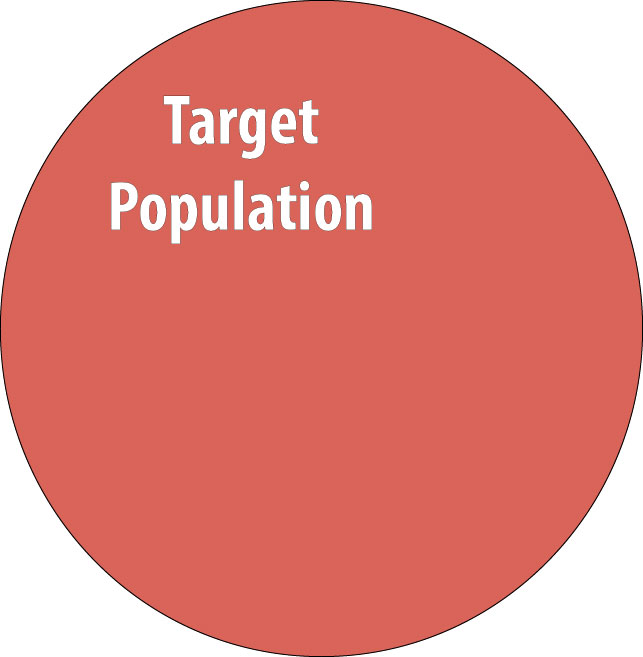
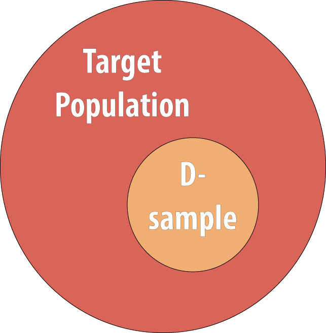
As discussed in chapter 1, we rarely conduct studies on entire populations because they are too big for it to be logistically feasible to study everyone in the population. Therefore we draw a sample and perform the study with the individuals in the sample. For a cohort study, since we will be calculating incidence, we must start with individuals who are at risk of the outcome. We thus draw a non-diseased sample from the target population:

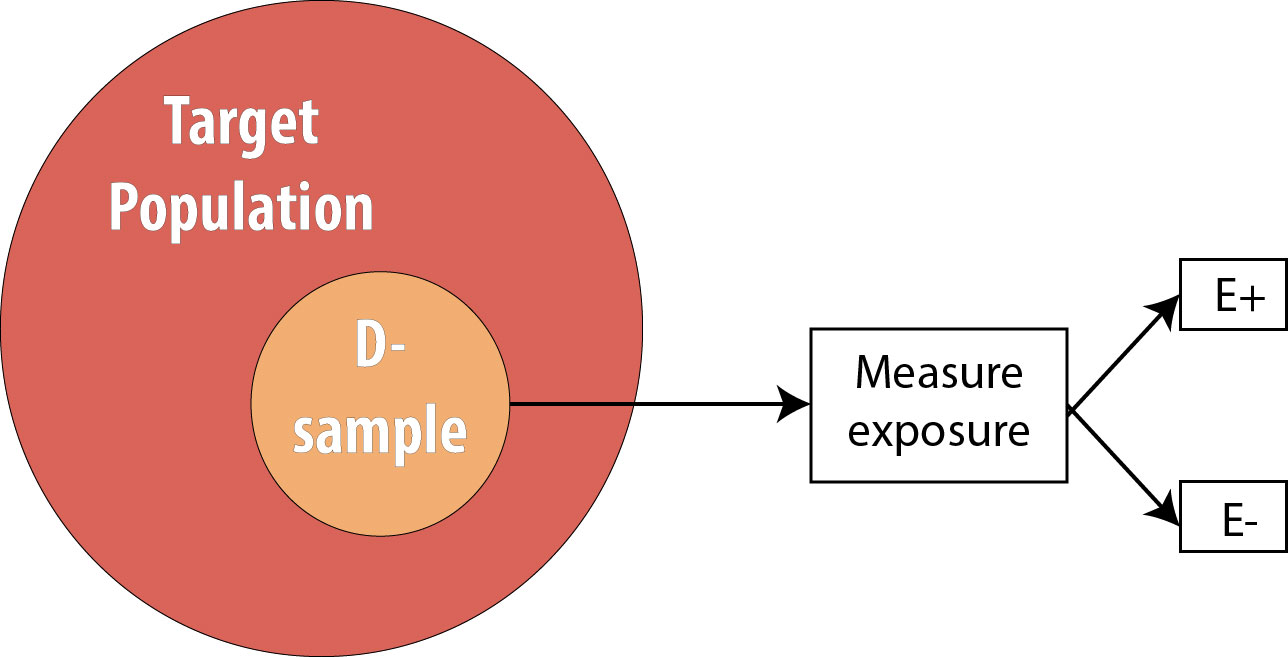
The next step is to assess the exposure status of the individuals in our sample and determine whether they are exposed or not:

After assessing which participants were exposed, our 2 x 2 table (using the 10-person smoking/HTN data example from above) would look like this:

By definition, at the beginning of a cohort study, everyone is still at risk of developing the disease, and therefore there are no individuals in the D+ column. In this hypothetical example, based on the data above, we will observe 5 cases of incident hypertension as the study progresses–but at the beginning, none of these cases have yet occurred.

We then follow the participants in our study for some length of time and observe incident cases as they arise.

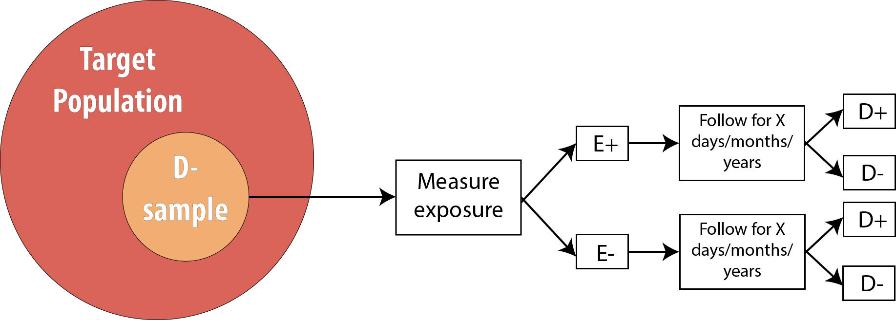
As mentioned in chapter 2, the length of follow-up varies depending on the disease process in question. For a research question regarding childhood exposure and late-onset cancer, the length of follow-up would be decades. For an infectious disease outbreak, the length of follow-up might be a matter of days or even hours, depending on the incubation period of the particular disease.

Assuming we are calculating incidence proportions (which use the number of people at risk in the denominator) in our cohort, our 2 × 2 table at the end of the smoking/HTN study would look like this:

It is important to recognize that when epidemiologists talk about a 2 × 2 table from a cohort study, they mean the 2 × 2 table at the end of the study—the 2 × 2 table from the beginning was much less interesting, as the D+ column was empty!

From this 2 × 2 table, we can calculate a number of useful measures, detailed below.

Calculating the Risk Ratio from the Hypothetical Smoking/Hypertension Cohort Study

We can also calculate the incidence only among exposed individuals:

I E+ = [latex]\frac{A}{(A+B)} = \frac{3}{4}[/latex] = 75 per 100 in 10 years

Likewise, we can calculate the incidence only among unexposed individuals:

I E- = [latex]\frac{C}{(C+D)} = \frac{2}{6}[/latex] = 33 per 100 in 10 years

Recall that our original goal with the cohort study was to see whether exposure is associated with disease. We thus need to compare the I E+ to the I E- . The most common way of doing this is to calculate their combined ratio:

Risk Ratio = [latex]\frac{I_{E+}}{I_{E-}} = \frac{\text{75 per 100 in 10 years}}{\text{33 per 100 in 10 years}}[/latex] = 2.27

Using ABCD notation, the formula for RR is:

[latex]\frac{\frac{A}{(A+B)}}{\frac{C}{(C+D)}}[/latex]

Note that risk ratios (RR) have no units, because the time-dependent units for the 2 incidences cancel out.

If the RR is greater than 1, it means that we observed more disease in the exposed group than in the unexposed group. Likewise, if the RR is less than 1, it means that we observed less disease in the exposed group than in the unexposed group. If we assume causality, an exposure with an RR < 1 is preventing disease, and an exposure with an RR > 1 is causing disease. The null value for a risk ratio is 1.0, which would mean that there was no observed association between exposure and disease. You can see how this would be the case—if the incidence was identical in the exposed and unexposed groups, then the RR would be 1, since x divided by x is 1.

Because the null value is 1.0, one must be careful if using the words higher or lower when interpreting RRs. For instance, an RR of 2.0 means that the disease is twice as common, or twice as high, in the exposed compared to the unexposed—not that it is 2 times more common, or 2 times higher , which would be an RR of 3.0 (since the null value is 1, not 0). If you do not see the distinction between these, don’t sweat it—just memorize and use the template sentence below, and your interpretation will be correct.

The correct interpretation of an RR is:

Using our smoking/HTN example:

The key phrase is times as high; with it, the template sentence works regardless of whether the RR is above or below 1. For an RR of 0.5, saying “0.5 times as high” means that you multiply the risk in the unexposed by 0.5 to get the risk in the exposed, yielding a lower incidence in the exposed—as one expects with an RR < 1.

If our cohort study instead used a person-time approach, the 2 x 2 table at the end of the study would have a column for sum of the person-time at risk (PTAR) :

Calculating the Rate Ratio from the Hypothetical Smoking/Hypertension Cohort Study

The interpretation is the same as it would be for the risk ratio; one just needs to substitute the word rate for the word risk :

Notice that the interpretation sentence still includes the duration of the study, even though some individuals (the 4 who developed hypertension) were censored before that time. This is because knowing how long people were followed for (and thus given time to develop disease) is still important when interpreting the findings. As discussed in chapter 2, 100 years of person-time can be accumulated in any number of different ways; knowing that the duration of the study was 10 years (rather than 1 year or 50 years) might make a difference in terms of how (or if) one applies the findings in practice.

“Relative Risk”

Both the risk ratio and the rate ratio are abbreviated RR . This abbreviation (and the risk ratio and/or rate ratio) is often referred to by epidemiologists as relative risk . This is an example of inconsistent lexicon in the field of epidemiology; in this book, I use risk ratio and rate ratio separately (rather than relative risk as an umbrella term) because it is helpful, in my opinion, to distinguish between studies using the population at risk vs. those using a person-time at risk approach. Regardless, a measure of association called RR is always calculated as incidence in the exposed divided by incidence in the unexposed.

Retrospective Cohort Studies

Throughout this book, I will focus on prospective cohort studies. One can also conduct a retrospective cohort study, mentioned here because public health and clinical practitioners will encounter retrospective cohort studies in the literature. In theory, a retrospective cohort study is conducted exactly like a prospective cohort study: one begins with a non-diseased sample from the target population, determines who was exposed, and “follows” the sample for x days/months/years, looking for incident cases of disease. The difference is that, for a retrospective cohort study, all this has already happened, and one reconstructs this information using existing records. The most common way to do retrospective cohort studies is by using employment records (which often have job descriptions useful for surmising exposure—for instance, the floor manager was probably exposed to whatever chemicals were on the factory floor, whereas human resource officers probably were not), medical records, or other administrative datasets (e.g., military records).

Continuing with our smoking/HTN 10-year cohort example, one might do a retrospective cohort using medical records as follows:

Go back to all the records from 10 years ago and determine who already had hypertension (these people are not at risk and are therefore not eligible) or otherwise does not meet the sample inclusion criteria
Determine, among those at risk 10 years ago, which individuals were smokers
Determine which members of the sample then developed hypertension during the intervening 10 years

Retrospective cohorts are analyzed just like prospective cohorts—that is, by calculating rate ratios or risk ratios. However, for beginning epidemiology students, retrospective cohorts are often confused with case-control studies; therefore we will focus exclusively on prospective cohorts for the remainder of this book. (Indeed, occasionally even seasoned scientists are confused about the differenc e!) i

Randomized Controlled Trials

The procedure for a randomized controlled trial (RCT) is exactly the same as the procedure for a prospective cohort, with one exception: instead of allowing participants to self-select into “exposed” and “unexposed” groups, the investigator in an RCT randomly assigns some participants (usually half) to “exposed” and the other half to “unexposed.” In other words, exposure status is determined entirely by chance. This is the type of study required by the Food and Drug Administration for approval of new drugs: half of the participants in the study are randomly assigned to the new drug and half to the old drug (or to a placebo, if the drug is intended to treat something previously untreatable). The diagram for an RCT is as follows:

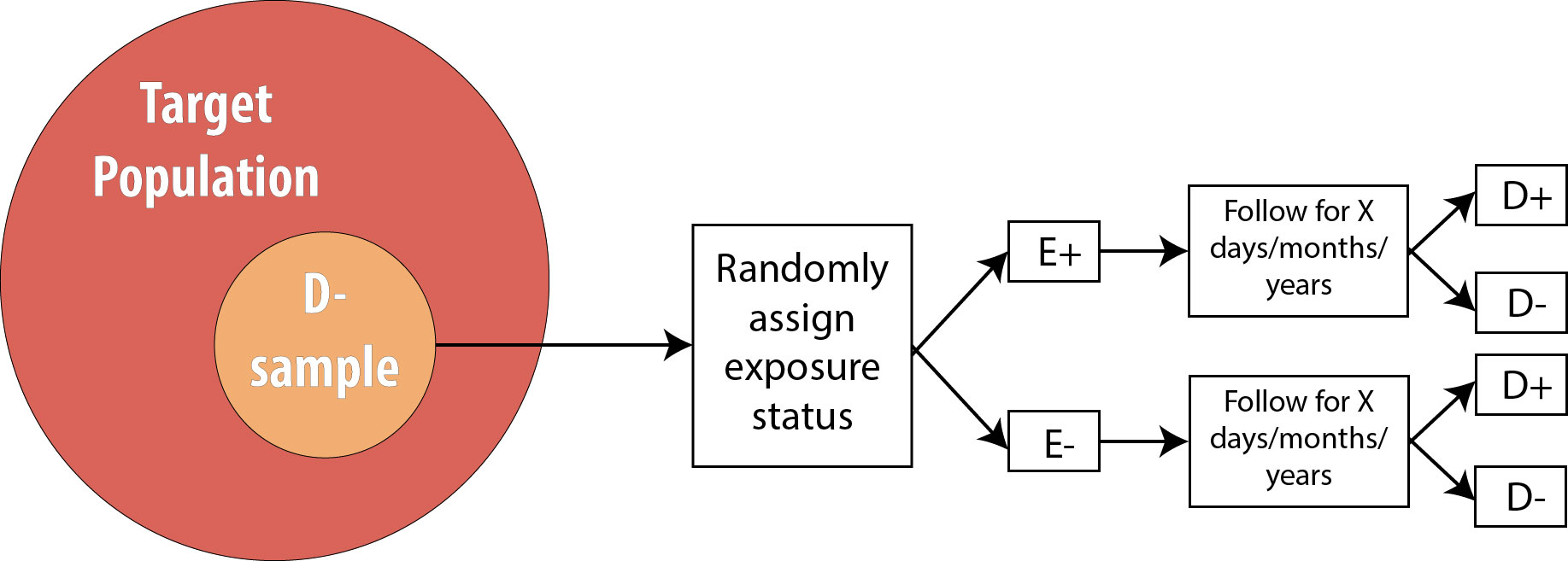
Note that the only difference between an RCT and a prospective cohort is the first box: instead of measuring existing exposures, we now tell people whether they will be exposed or not. We are still measuring incident disease, and we are therefore still calculating either the risk ratio or the rate ratio.

Observational versus Experimental Studies

Cohort studies are a subclass of observational studies , meaning the researcher is merely observing what happens in real life—people in the study self-select into being exposed or not depending on their personal preferences and life circumstances. The researcher then measures and records a given person’s level of exposure. Cross-sectional and case-control studies are also observational. Randomized controlled trials, on the other hand, are experimental studies—the researcher is conducting an experiment that involves telling people whether they will be exposed to a condition or not (e.g., to a new drug).

Studies That Use Prevalence Data

Following participants while waiting for incident cases of disease is expensive and time-consuming. Often, epidemiologists need a faster (and cheaper) answer to their question about a particular exposure/disease combination. One might instead take advantage of prevalent cases of disease, which by definition have already occurred and therefore require no wait. There are 2 such designs that I will cover: cross-sectional studies and case-control studies . For both of these, since we are not using incident cases, we cannot calculate the RR, because we have no data on incidence. We instead calculate the odds ratio (OR) .

Cross-sectional

Cross-sectional studies are often referred to as snapshot or prevalence studies: one takes a “snapshot” at a particular point in time, determining who is exposed and who is diseased simultaneously. The following is a visual:

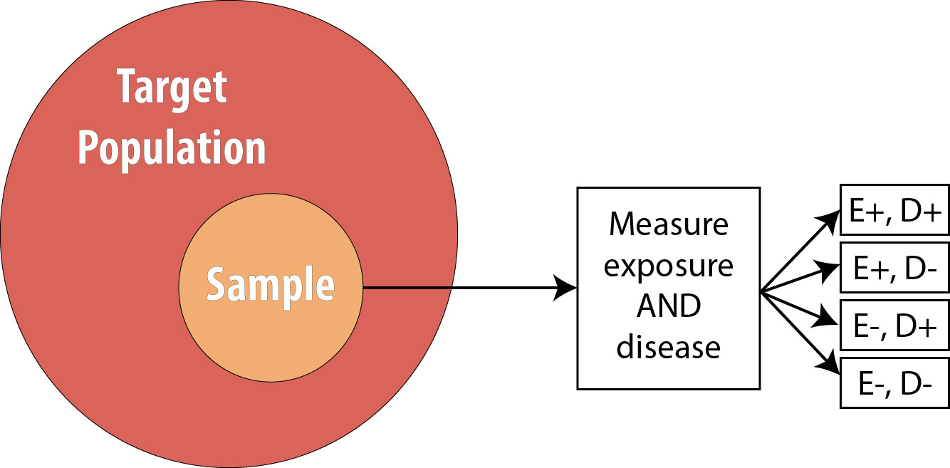
Note that the sample is now no longer composed entirely of those at risk because we are using prevalent cases—thus by definition, some proportion of the sample will be diseased at baseline . As mentioned, we cannot calculate the RR in this scenario, so instead we calculate the OR.

Calculating the Odds Ratio from the Hypothetical Smoking/Hypertension Cross-Sectional Study

The formula for OR for a cross-sectional study is:

OR = [latex]\frac{\text{odds of disease in the exposed group}}{\text{odds of disease in the unexposed group}}[/latex]

The odds of an event is defined statistically as the number of people who experienced an event divided by the number of people who did not experience it. Using 2 × 2 notation, the formula for OR is:

OR = [latex]\frac{\frac{A}{B}}{\frac{C}{D}} = \frac{AD}{BC}[/latex]

For our smoking/HTN example, if we assume those data came from a cross-sectional study, the OR would be:

OR = [latex]\frac{\frac{3}{1}}{\frac{2}{4}} = \frac{3*4}{2*1}[/latex] = 6.0

Again there are no units.

The interpretation of an OR is the same as that of an RR, with the word odds substituted for risk :

Note that we now no longer mention time, as these data came from a cross-sectional study, which does not involve time. As with interpretation of RRs, ORs greater than 1 mean the exposure is more common among diseased, and ORs less than 1 mean the exposure is less common among diseased. The null value is again 1.0.

For 2 x 2 tables from cross-sectional studies, one can additionally calculate the overall prevalence of disease as

Finally, some authors will refer to the OR in a cross-sectional study as the prevalence odds ratio— presumably, just as a reminder that cross-sectional studies are conducted on prevalent cases. The calculation of such a measure is exactly the same as the OR as presented above.

OR versus RR

As you can see from the (hypothetical) example data in this chapter, the OR will always be further from the null value than the RR. The more common the disease, the more this is true. If the disease has a prevalence of about 5% or less, then the OR does provide a close approximation of the RR; however, as the disease in question becomes more common (as in this example, with a hypertension prevalence of 40%), the OR deviates further and further from the RR.

Occasionally, you will see a cohort study (or very rarely, an RCT) that reports the OR instead of the RR. Technically this is not correct, because cohorts and RCTs use incident cases, so the best choice for a measure of association is the RR. However, one common statistical modeling technique—logistic regression—automatically calculates ORs. While it is possible to back-calculate the RR from these numbers, often investigators do not bother and instead just report the OR. This is troublesome for a couple of reasons: first, it is easier for human brains to interpret risks as opposed to odds, and therefore risks should be used when possible; and second, cohort studies and RCTs almost always have relatively common outcomes (see chapter 9), thus reporting the OR makes it seem as if the exposure is a bigger problem (or a better solution, if OR < 1) than it “really” is.

Case-Control

The final type of epidemiologic study that is commonly used is the case-control study. It also begins with prevalent cases and thus is faster and cheaper than longitudinal (prospective cohort or RCT) designs. To conduct a case-control study, one first draws a sample of diseased individuals (cases):

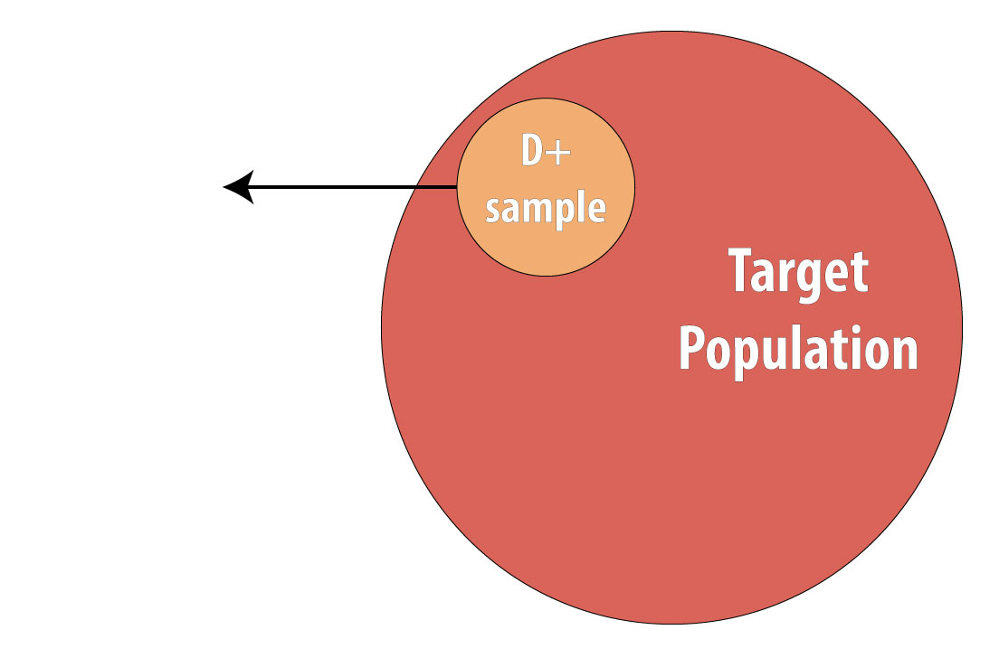
Then a sample of nondiseased individuals (controls):

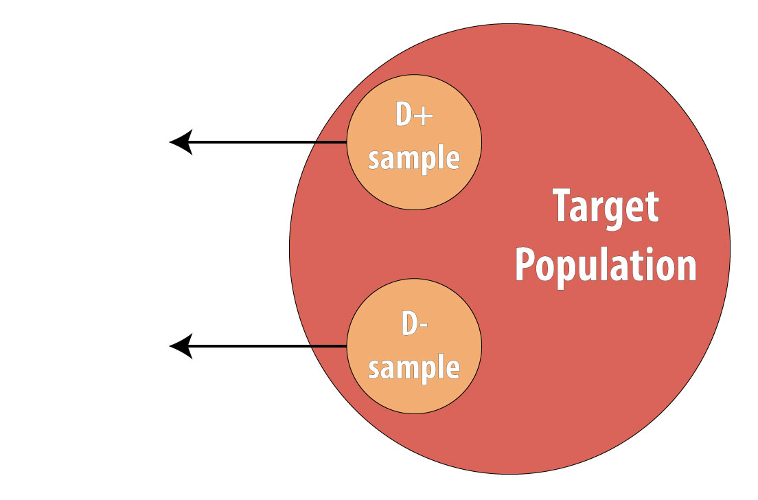
First and foremost, note that both cases and controls come from the same underlying population. This is extremely important, lest a researcher conduct a biased case-control study (see chapter 9 for more on this). After sampling cases and controls, one measures exposures at some point in the past . This might be yesterday (for a foodborne illness) or decades ago (for osteoporosis):

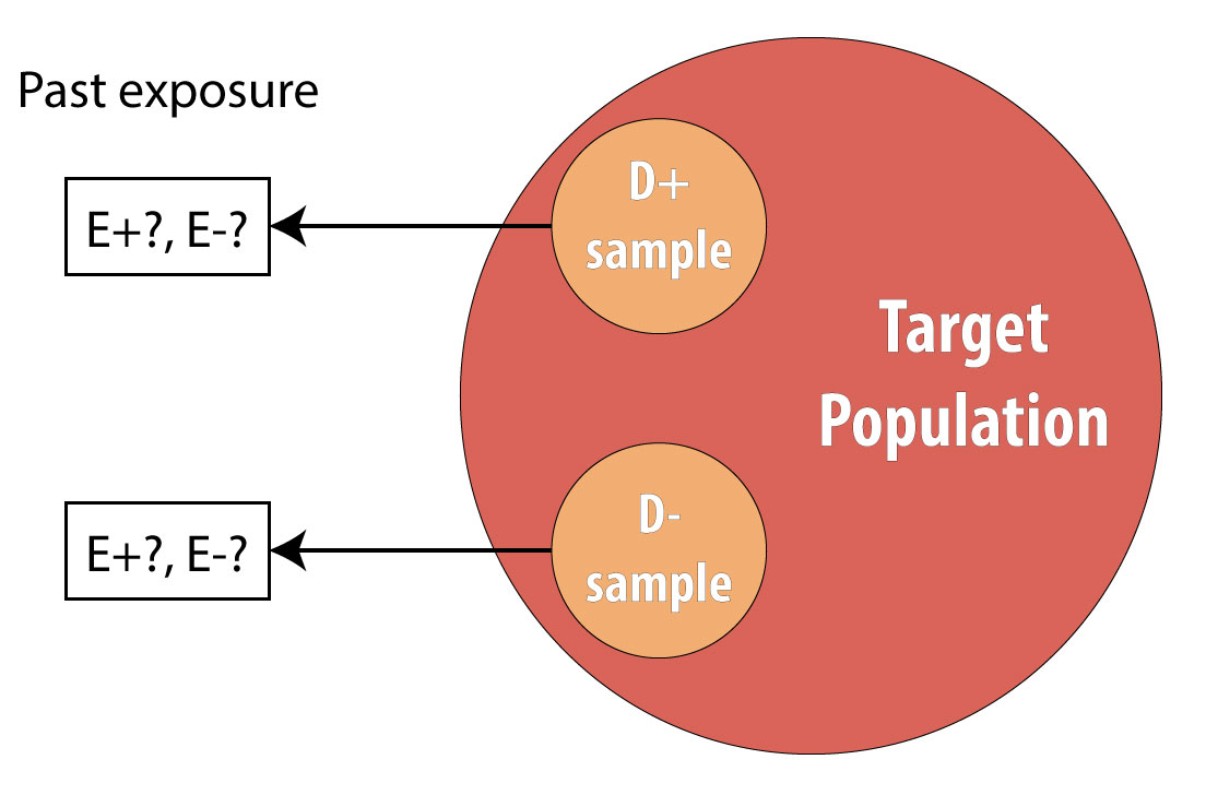
Again, we cannot calculate incidence because we are using prevalent cases, so instead we calculate the OR in the same manner as above. The interpretation is identical, but now we must refer to the time period because we explicitly looked at past exposure data:

Note, however, that one cannot calculate the overall sample prevalence using a 2 × 2 table from a case-control study, because we artificially set the prevalence in our sample (usually at 50%) by deliberately choosing individuals who were diseased for our cases.

Exposure OR versus Disease OR

Technically, for a case-control study, one calculates the disease OR rather than the exposure OR (which is presented under cross-sectional studies). In other words, since in case-control studies we begin with disease, we are calculating the odds of being exposed among those who are diseased compared to the odds of being exposed among those who are not diseased:

OR disease [latex]= \frac{\left(A/{C}\right)}{\left(B/{D}\right)} = \frac{AD}{BC}[/latex]

The exposure odds ratio, you will remember, calculates the odds of being diseased among those who are exposed, compared to the odds of being diseased among those who are unexposed:

OR exposure [latex]= \frac{\left(A/{B}\right)}{\left(C/{D}\right)} = \frac{AD}{BC}[/latex]

In advanced epidemiology classes, one is expected to appreciate the nuances of this difference and to articulate the rationale behind it. However, since both the exposure and the disease odds ratios simplify to the same final equation, here we will not differentiate between them. The interpretation is the same: an OR > 1 means that disease is more common in the exposed group (or exposure is more common in the diseased group—same thing), and an OR < 1 means that disease is less common in the exposed group (or exposure is less common in the diseased group—again, same thing).

Risk Difference

RR and OR are known as relative or ratio measures of association for obvious reasons. These measures can be misleading, however, if the absolute risks (incidences) are small. [2] For example, if a cohort study was done, and investigators observed an incidence in the exposed of 1 per 1,000,000 in 20 years and an incidence in the unexposed, and an incidence in the unexposed of 2 per 1,000,000 in 20 years, the RR would be 0.5: there is a 50% reduction in disease in the exposed group. Break out the public health intervention! However, this ratio measure masks an important truth: the absolute difference in risk is quite small: 1 in a million.

To address this issue, epidemiologists sometimes calculate instead the risk difference instead:

RD = I E+ – I E-

Unfortunately, this absolute measure of association is not often seen in the literature, perhaps because interpretation implies causation more explicitly or because it is more difficult to control for confounding variables (see chapter 7) when calculating difference measures.

Regardless, in our smoking/HTN example, the RD is:

RD = I E+ – I E- = 75 per 100 in 10 years – 33 per 100 in 10 years = 42 per 100 in 10 years

Note that the RD has the same units as incidence, since units do not cancel when subtracting. The interpretation is as follows:

Over 10 years, the excess number of cases of HTN attributable to smoking is 42; the remaining 33 would have occurred anyway.

You can see how this interpretation assigns a more explicitly causal role to the exposure.

More common (but still not nearly as common as the ratio measures) are a pair of measures derived from the RD: the attributable risk (AR) and the number needed to treat/number needed to harm (NNT/NNH).

The AR is calculated as RD/I E+ . Here,

AR = 42 per 100 in 10 years / 75 per 100 in 10 years = 56%

Interpretation:

56% of cases can be attributed to smoking, and the rest would have happened anyway.

Again this implies causality; furthermore, because diseases all have more than one cause (see chapter 10), the ARs for each possible cause will sum to well over 100%, making this measure less useful.

Finally, calculating NNT/NNH (both of which are similar, with the former being for preventive exposures and the latter for harmful ones) is simple:

In our example,

NNH = 1 / 42 per 100 per 10 years = 1/0.42 per 10 years = 2.4

Over 10 years, for every 2.4 smokers, 1 will develop hypertension.

For a protective exposure, the NNT (commonly used in clinical circles) is interpreted as the number you need to treat in order to prevent one case of a bad outcome. For harmful exposures, as in our smoking/HTN example, it is the number needed to be exposed to cause one bad outcome. For many drugs in common use, the NNTs are in the hundreds or even thousands. [iii] [iv]

Conclusions

Epidemiologic data are often summarized in 2 × 2 tables. There are 2 main measures of association commonly used in epidemiology: the risk ratio/rate ratio (relative risk) and the odds ratio. The former is calculated for study designs that collect data on incidence: cohorts and RCTs. The latter is calculated for study designs that use prevalent cases: cross-sectional studies and case-control studies. Absolute measures of association (e.g., risk difference) are not seen as often in epidemiologic literature, but it is nonetheless always important to keep the absolute risks (incidences) in mind when interpreting results.

Below is a table summarizing the concepts from this chapter:

i. Bodner K, Bodner-Adler B, Wierrani F, Mayerhofer K, Fousek C, Niedermayr A, Grünberger. Effects of water birth on maternal and neonatal outcomes. Wien Klin Wochenschr . 2002;114(10-11):391-395. ( ↵ Return )

ii. Declercq E. The absolute power of relative risk in debates on repeat cesareans and home birth in the United States. J Clin Ethics . 2013;24(3):215-224.

iii. Mørch LS, Skovlund CW, Hannaford PC, Iversen L, Fielding S, Lidegaard Ø. Contemporary hormonal contraception and the risk of breast cancer. N Engl J Med . 2017;377(23):2228-2239. doi:10.1056/NEJMoa1700732 ( ↵ Return )

iv. Brisson M, Van de Velde N, De Wals P, Boily M-C. Estimating the number needed to vaccinate to prevent diseases and death related to human papillomavirus infection. CMAJ Can Med Assoc J . 2007;177(5):464-468. doi:10.1503/cmaj.061709 ( ↵ Return )

These 4 study designs are the basis for nearly all others (e.g., case-crossover studies are a subtype of case-control studies). A few additional designs are covered in chapter 9, but a firm understanding of the 4 designs covered in this chapter will set beginning epidemiology students up to be able to critically read essentially all of the literature. ↵
Declercq E. The absolute power of relative risk in debates on repeat cesareans and home birth in the United States. J Clin Ethics . 2013;24(3):215-224 ↵

Refers to a situation wherein exposed individuals have either more or less of the disease of interest (or diseased individuals have either more or less of the exposure of interest) than unexposed individuals.

Quantifies the degree to which a given exposure and outcome are related statistically. Implies nothing about whether the association is causal. Examples of measures of association are odds ratios , risk ratios , rate ratios , risk differences , etc.

A measure of disease frequency that quantifies occurrence of new disease. There are two types, incidence proportion and incidence rate . Both of these have “number of new cases” as the numerator; both can be referred to as just “incidence.” Both must include time in the units, either actual time or person-time. Also called absolute risk .

A measure of disease frequency that quantifies existing cases. The numerator is "all cases" and the denominator is "the number of people in the population." Usually expressed as a percent unless the prevalence is quite low, in which case write it as "per 1000" or "per 10,000" or similar. There are no units for prevalence, though it is understood that the number refers to a particular point in time.

A convenient way for epidemiologists to organize data, from which one calculates either measures of association or test characteristics .

High blood pressure, often abbreviated HTN.

See cohort study .

An intervention (experimental) study. Just like a prospective cohort except that the investigator tells people randomly whether they will be exposed or not. So, grab an at-risk (non-diseased) sample from the target population , randomly assign half of them to be exposed and half to be non-exposed, then follow looking for incident cases of disease. The correct measure of association is the risk ratio or rate ratio . If done with a large enough sample, RCTs will be free from confounders (this is their major strength), because all potential co-variables will be equally distributed between the two groups (thus making it so that no co-variables are associated with the exposure, a necessary criterion for a confounder). Note that the ‘random’ part is in assigning the exposure, NOT in getting a sample (it does not need to be a ‘random sample’). RCTs are often not do-able because of ethical concerns.

The start of a cohort study or randomized controlled trial .

An observational design. Usually prospective, in which case one selects a sample of at-risk (non-diseased) people from the target population , assesses their exposure status, and then follows them over time looking for incident cases of disease. Because we measure incidence , the usual measure of association is either the risk ratio or the rate ratio , though occasionally one will see odds ratios reported instead. If the exposure under study is common (>10%), one can just select a sample from the target population; however, if the exposure is rare, then exposed persons are sampled deliberately. (Cohort studies are the only design available for rare exposures.) This whole thing can be done in a retrospective manner if one has access to existing records (employment or medical records, usually) from which one can go back and "create" the cohort of at-risk folks, measure their exposure status at that time, and then "follow" them and note who became diseased.

The group about which we want to be able to say something. One only very rarely is able to enroll the entire target population into a study (since it would be millions and millions of people), and so instead we draw a sample , and do the study with them. In epidemiology we often don't worry about getting a "random sample"--that's necessary if we're asking about opinions or health behaviors or other things that might vary widely by demographics, but not if we're measuring disease etiology or biology or something else that will likely not vary widely by demographics (for instance, the mechanism for developing insulin resistance is the same in all humans).

The group actually enrolled in a study. Hopefully the sample is sufficiently similar to the target population that we can say something about the target population , based on results from our sample. In epidemiology we often don’t worry about getting a “random sample”–that’s necessary if we’re asking about opinions or health behaviours or other things that might vary widely by demographics, but not if we’re measuring disease etiology or biology or something else that will likely NOT vary widely by demographics (for instance, the mechanism for developing insulin resistance is likely the same in all humans). Nonetheless, if the sample is different enough than the target population, that is a form of selection bias , and can be detrimental in terms of external validity .

The amount of time between an exposure and the onset of symptoms. Roughly, the induction period plus the latent period .

A measure of disease frequency . The numerator is "number of new case" and the denominator is "the number of people who were at risk at the start of follow-up." Sometimes if the denominator is unknown, you can substitute the population at the mid-point of follow-up (an example would be the incidence of ovarian cancer in Oregon. We would know how many new cases popped up in a given year, via cancer surveillance systems. To estimate the incidence proportion, we could divide by the number of women living in Oregon on July 1 of that year. This of course is only an estimate of the true incidence proportion, as we don't know exactly how many women lived here, nor do we know which of them might not have been at risk of ovarian cancer.) The units for incidence proportion are "per unit time." You can adjust this if necessary (ie if you follow people for 1 month, you can multiply by 12 to estimate the incidence for 1 year). You can (read: should) also adjust the final answer so that it looks "nice." For instance, 13.6/100,000 in 1 year is easier to comprehend than 0.000136 in 1 year. Also called risk and cumulative incidence .

A measure of association calculated for studies that observe incident cases of disease ( cohorts or RCTs ). Calculated as the incidence proportion in the exposed over the incidence proportion in the unexposed, or A/(A+B) / C/(C+D), from a standard 2x2 table . Note that 2x2 tables for cohorts and RCTs show the results at the end of the study--by definition, at the beginning, no one was diseased. See also rate ratio and relative risk . Abbreviated RR.

The value taken by a measure of association if the exposure and disease are not related. Is equal to 1.0 for relative measures of association , and equal to 0.0 for absolute measures of association .

For participants enrolled in a cohort study or randomized controlled trial , this is the amount of time each person spent at risk of the disease or health outcome. A person stops accumulating person-time at risk (usually shortened to just "person-time") when: (1) they are lost to follow-up; (2) they die (or otherwise not become a risk) of something else other than the disease under study (ie they die of a competing risk ); (3) they experience the disease or health outcome under study (now they are an incident case ); or (4) the study ends. Each person enrolled in such a study could accumulate a different amount of person-time at risk.

A measure of disease frequency . The numerator is "number of new cases." The denominator is "sum of the person-time at risk ." The units for incidence rate are "per person-[time unit]", usually but not always person-years. You can (and should) adjust the final answer so that it looks "nice." For instance, instead of 3.75/297 person-years, write 12.6 per 1000 person-years. Also called incidence density.

Stopped being followed-up, in this case because they got the disease and so were no longer contributing person-time at risk. The 6 individuals who did not develop disease were also censored, either at the end of the 10 years, or potentially earlier if any individuals died (a competing risk) or were otherwise lost to follow-up.

All study designs in which participants choose their own exposure groups. Includes cohorts , case-control , cross-sectional . Basically, includes all designs other than randomized controlled trial .

An observational study design in which one takes a sample from the target population, assesses their exposure and disease status all at that one time. One is capturing prevalent cases of disease; thus the odds ratio is the correct measure of association. Cross-sectional studies are good because they are quick and cheap; however, one is faced with the chicken-egg problem of not knowing whether the exposure came before the disease.

An observational study that begins by selecting cases (people with the disease) from the target population . One then selects controls (people without the disease)–importantly, the controls must come from the same target population as cases (so, if they suddenly developed the disease, they’d be a case). Also, selection of both cases and controls is done without regard to exposure status. After selecting both cases and controls, one then determines their previous exposure(s). This is a retrospective study design, and as such, more prone to things like recall bias than prospective designs. Case-control studies are necessary if the disease is rare and/or if the disease has a long induction period . The only appropriate measure of association is the odds ratio , because one cannot measure incidence in a case-control study.

A measure of association , used in study designs that deal with prevalent cases of disease ( case-control , cross-sectional ). Calculated as AD/BC, from a standard 2x2 table . Abbreviated OR.

At the start of a study.

See Incidence .

A measure of association calculated fundamentally by subtraction. See also risk difference .

Share This Book

Do Case-Control Studies Always Estimate Odds Ratios?

PMID: 32889542
PMCID: PMC7850067
DOI: 10.1093/aje/kwaa167

Case-control studies are an important part of the epidemiologic literature, yet confusion remains about how to interpret estimates from different case-control study designs. We demonstrate that not all case-control study designs estimate odds ratios. On the contrary, case-control studies in the literature often report odds ratios as their main parameter even when using designs that do not estimate odds ratios. Only studies using specific case-control designs should report odds ratios, whereas the case-cohort and incidence-density sampled case-control studies must report risk ratio and incidence rate ratios, respectively. This also applies to case-control studies conducted in open cohorts, which often estimate incidence rate ratios. We also demonstrate the misinterpretation of case-control study estimates in a small sample of highly cited case-control studies in general epidemiologic and medical journals. We therefore suggest that greater care be taken when considering which parameter is to be reported from a case-control study.

Keywords: case-control studies; control sampling; incidence rate ratio; odds ratio; risk ratio.

Case-Control Studies*
Data Interpretation, Statistical*
Odds Ratio*
Research Design*

EP717 Module 5 - Epidemiologic Study Designs – Part 2:

Case-control studies.

Page:
1
| 2
| 3
| 4
| 5
| 6
| 7

A Nested Case-Control Study

Interpretation of the odds ratio, test yourself, recap of case-control design.

Now consider a hypothetical prospective cohort study among 89,949 women in whom the investigators took blood samples and froze them at baseline for possible future use. After following the cohort for 12 years the investigators wanted to investigate a possible association between the pesticide DDT and breast cancer. Since they had frozen blood samples collected at baseline, they had the option of having the samples tested for DDT levels. If they had done this, the table below shows what they would have found.

If they had had this data, they could have calculated the risk ratio:

RR = (360/13,636) / (1,079/76,313) = 1.87

However, the cost of analyzing each sample for DDT was $20, and to analyze all of them would have cost close to $1.8 million. So, like the previous study, the exposure data was very costly.

Although this was a prospective cohort study, we could regard the cohort as a source population and conduct a case-control study drawing samples from the cohort . We could, for example, analyze the blood samples on all of the women who had developed breast cancer during the 12 year follow up and on 2,878 randomly selected samples from the women without breast cancer (i.e., twice as many controls as cases). This would be described as a nested case-control study , i.e., nested within a cohort study.

The results might have looked like this:

Odds Ratio = (a/c) / (b/d) = (360/1,079) / (432/2,446)

= 1.89 during the 12 year follow up study

So, they could achieve an odds ratio that is very close to what the risk ratio would have been at a much lower cost: (1,439+2,878) x $20 = $86,340.

The odds ratio is a legitimate measure of association, and, when the outcome of interest is uncommon, it provides a good estimate of what the risk ratio would have been if a cohort study had been possible. When looking at increasingly common outcomes, the odds ratio gives estimates that are more extreme than the risk ratio, i.e., further away from the null value.

Not surprisingly, the interpretation of an odds is therefore similar to the interpretation of a risk ratio.

The null value (no difference) is 1.0.
Odds ratios > 1 suggest an increase in risk
Odds ratios < 1 suggest a decrease in risk

The odds ratio above would be interpreted as follows:

"Women with high DDT blood levels at baseline had 1.89 times the odds of developing breast cancer compared to women with low blood levels of DDT during the 12 year observation period."

Calculate the odds ratio for the association between playing video games and development of hypertension. Interpret the odds ratio you calculate in a sentence. See if you can do both of these correctly before looking at the answer.

return to top | previous page | next page

User Preferences

Content preview.

Arcu felis bibendum ut tristique et egestas quis:

Keyboard Shortcuts

9.5 - example 9-3 : odds ratios from a case/control study, example 9-3 section .

Suppose your study design is an unmatched case-control study with equal numbers of cases and controls .

If 30% of the population is exposed to a risk factor, what is the number of study subjects (assuming an equal number of cases and controls in an unmatched study design) necessary to detect a hypothesized odds ratio of 2.0? Assume 90% power $\alpha=0.05$.

Here are the hypotheses being tested:

Null hypothesis

$H_0\colon \text{incidence}_{1}^* \le \text{incidence}_{2}^*$

Alternative hypothesis

$H_A\colon \text{incidence}_{1}^* / \text{incidence}_{2}^*=\lambda^*$

$\lambda^*\gt0$

$\text{Disease incidence}_1^*=p(\text{Exposed|Case})$

$\text{Disease incidence}_2^*=p(\text{Not Exposed|Control})$

The resulting sample size formula is:

$n=\dfrac{(r+1)(1+(\lambda -1)P)^{2}}{rP^{2}(P-1)^{2}(\lambda -1)P)^{2}}\left [ z_{\alpha}\sqrt{(r+1)p_{c}^{*}(1-p_{c}^{*})} + z_{\beta}\sqrt{\frac{\lambda P(1-P)}{\left [ 1+(\lambda-1)P \right ]^{2}}+rP(1-P)} \right ]^{2}$

$p_{c}^{*}=\dfrac{P}{r+1}\left ( \dfrac{r\lambda}{1+(\lambda -1)P}+1 \right )$

Table B.10. Total sample size requirements (for the two groups combined) for unmatched case-control studies with equal numbers of cases and controls with equal numbers in each group

Need a hint?

We have considered three typical epidemiologic research designs. You might also ask these questions:

Should the number of controls match the number of cases? Should multiple controls be used for each case?

Observe the power curve below:

Power increases but at a decreasing rate as the ratio of controls/cases increases. Little additional power is gained at ratios higher than four controls/cases. There is little benefit to enrolling a greater ratio of controls to cases.

from Woodward, M. Epidemiology Study Design and Analysis . Boca Raton: Chapman and Hall, 1999, p.265

Under what circumstances would it be recommended to enroll a large number of controls compared to cases?

Perhaps the small gain in power is worthwhile if the cost of a Type II error is large and the expense of obtaining controls is minimal, such as selecting controls with covariate information from a computerized database. If you must physically locate and recruit the controls, set up clinic appointments, run diagnostic tests, and enter data, the effort of pursuing a large number of controls quickly offsets any gain. You would use a one-to-one or two-to-one range. The bottom line is there is little additional power beyond a four-to-one ratio.

What if there is a Limited Number of Total Subjects for Case-Control Studies?

Sometimes the total number of subjects is limited (e.g., you have limited funds and the cost associated with each case is equal to the cost associated with a control). This graph illustrates power as related to the ratio of the controls to cases.

from Woodward, M. Epidemiology Study Design and Analysis . Boca Raton: Chapman and Hall, 1999, p.358

There is maximum power with a one-to-one ratio of controls to cases. If you are limited in the number of people that can be enrolled in a study, match cases to controls in a one-to-one fashion.

What about Matched Case-Control Studies?

In matched case/control study designs, useful data come from only the discordant pairs of subjects. Useful information does not come from the concordant pairs of subjects. Matching of cases and controls on a confounding factor (e.g., age, sex) may increase the efficiency of a case-control study, especially when the moderator's minimal number of controls are rejected.

The sample size for matched study designs may be greater or less than the sample size required for similar unmatched designs because only the pairs discordant on exposure are included in the analysis. The proportion of discordant pairs must be estimated to derive sample size and power. The power of matched case/control study design for a given sample size may be larger or smaller than the power for an unmatched design.

Formula for sample size calculation for matched case-control study:

$n=\dfrac{(r+1)(1+(\lambda -1)P)^{2}}{rP^{2}(P-1)^{2}(\lambda -1)^{2}}\left [ z_{\alpha}\sqrt{(r+1)p_{c}^{*}} + z_{\beta}\sqrt{\frac{\lambda P(1-P)}{\left [ 1+(\lambda-1)P \right ]^{2}}+rP(1-P)} \right ]^{2}$

P = prevalence of exposure among the population $\lambda$ = estimated relative risk r = ratio of cases to controls

- Google Chrome

Intended for healthcare professionals

Search form

Use of progestogens and the risk of intracranial meningioma: national case-control study

This article has a correction. Please see:

Objective To assess the risk of intracranial meningioma associated with the use of selected progestogens.

Design National case-control study.

Setting French National Health Data System (ie, Système National des Données de Santé ).

Participants Of 108 366 women overall, 18 061 women living in France who had intracranial surgery for meningioma between 1 January 2009 and 31 December 2018 (restricted inclusion periods for intrauterine systems) were deemed to be in the case group. Each case was matched to five controls for year of birth and area of residence (90 305 controls).

Main outcome measures Selected progestogens were used: progesterone, hydroxyprogesterone, dydrogesterone, medrogestone, medroxyprogesterone acetate, promegestone, dienogest, and intrauterine levonorgestrel. For each progestogen, use was defined by at least one dispensation within the year before the index date (within three years for 13.5 mg levonorgestrel intrauterine systems and five years for 52 mg). Conditional logistic regression was used to calculate odds ratio for each progestogen meningioma association.

Results Mean age was 57.6 years (standard deviation 12.8). Analyses showed excess risk of meningioma with use of medrogestone (42 exposed cases/18 061 cases (0.2%) v 79 exposed controls/90 305 controls (0.1%), odds ratio 3.49 (95% confidence interval 2.38 to 5.10)), medroxyprogesterone acetate (injectable, 9/18 061 (0.05%) v 11/90 305 (0.01%), 5.55 (2.27 to 13.56)), and promegestone (83/18 061 (0.5%) v 225/90 305 (0.2 %), 2.39 (1.85 to 3.09)). This excess risk was driven by prolonged use (≥one year). Results showed no excess risk of intracranial meningioma for progesterone, dydrogesterone, or levonorgestrel intrauterine systems. No conclusions could be drawn concerning dienogest or hydroxyprogesterone because of the small number of individuals who received these drugs. A highly increased risk of meningioma was observed for cyproterone acetate (891/18 061 (4.9%) v 256/90 305 (0.3%), odds ratio 19.21 (95% confidence interval 16.61 to 22.22)), nomegestrol acetate (925/18 061 (5.1%) v 1121/90 305 (1.2%), 4.93 (4.50 to 5.41)), and chlormadinone acetate (628/18 061 (3.5%) v 946/90 305 (1.0%), 3.87 (3.48 to 4.30)), which were used as positive controls for use.

Conclusions Prolonged use of medrogestone, medroxyprogesterone acetate, and promegestone was found to increase the risk of intracranial meningioma. The increased risk associated with the use of injectable medroxyprogesterone acetate, a widely used contraceptive, and the safety of levonorgestrel intrauterine systems are important new findings.

Introduction

Meningiomas account for 40% of primary tumours of the central nervous system. 1 2 The incidence of meningioma in the United States is 9.5 per 100 000 person years. 2 Meningiomas are mostly slow growing, histologically benign tumours but can nevertheless compress adjacent brain tissue and thus patients may require surgical decompression. 3 The incidence of meningiomas increases with age, rising sharply after the age of 65 years. Conversely, meningiomas are rare before the age of 35. Other recognised risk factors for meningioma are being female, intracranial exposure to ionising radiation, neurofibromatosis type 2 2 , and, as shown only recently, prolonged use (≥one year) to high doses of three potent progestogens: cyproterone acetate, 4 5 chlormadinone acetate, 4 and nomegestrol acetate. 4

The link between female sexual hormones, in particular progesterone, and intracranial meningioma is biologically plausible. 6 Progesterone receptors are present in more than 60% of meningiomas 7 and the volume of these tumours has been observed to increase during pregnancy and to decrease post partum. 8 However, previous pregnancy does not appear to be an unequivocal risk factor for meningioma. 9 Studies have also shown a link, albeit a weak one, between breast cancer and meningiomas. 10

No significant association between exogenous female hormones and risk of meningioma has been shown to date for hormonal contraceptives (either combined or progestogen only pills). 11 12 Additionally, data for hormone replacement treatment for menopause are contradictory. Several studies have shown a slight excess risk of meningioma associated with the use of hormone replacement treatment for menopause, 11 13 whereas others have reported no deleterious effects of these molecules. 14 By contrast, the excess risk of meningioma observed with the use of high doses of cyproterone acetate among cis women, men, and trans women has been shown to be very high 5 15 16 and somewhat lower, but still substantial, for chlormadinone acetate and nomegestrol acetate. 4 Discontinuation of each of these three progestogens generally leads to a reduction in meningioma volume, 17 18 which avoids the need for surgery and its associated risk of complications for most patients.

Whether progestogens other than these three oral progestogens at high doses have a similar effect depending on their route of administration is still unknown. Our study aimed to assess the real-life risk of intracranial meningioma associated with the use of progestogens from an extensive list (progesterone, hydroxyprogesterone, dydrogesterone, medrogestone, medroxyprogesterone acetate, promegestone, dienogest, and levonorgestrel intrauterine systems) with different routes of administration (oral, percutaneous, intravaginal, intramuscular, and intrauterine). Although some of the progestogens studied are used in France (promegestone) or in only a few countries (medrogestone), others are widely used worldwide in various doses and for various indications (progesterone, levonorgestrel, hydroxyprogesterone, medroxyprogesterone) (supplementary table A). Certain progestogens may also be risky at some doses when used over a long period of time, but not at lower doses or when used for a short period of time. Our secondary objectives were to describe the characteristics of the women who were in the cases group (age, grade, and anatomical location of the meningiomas) and to approximate the number of surgically treated meningiomas attributable to the use of the concerned progestogens.

Study design and data source

This observational population based study used data derived from the French national health data system ( Système National des Données de Santé (SNDS)). Given the analysis of multiple exposure situations (different exposure definitions and lookback periods) in our study, we opted for a case-control design rather than a cohort study, thus including long term users of the considered medications. 19

The SNDS database contains information on all health spending reimbursements for over 99% of the population residing in France and is linked to the French hospital discharge database. 20 SNDS is currently one of the largest healthcare databases in the world and is widely used in pharmacoepidemiological studies. 4 5 21 22 23 24

Definition of cases and selection of controls

The eligible cases in this study were women residing in France of all ages who underwent surgery for intracranial meningioma between 1 January 2009, and 31 December 2018. For each case, the start date of the corresponding admission to hospital marked the index date. Women with a pregnancy beginning in the two years before the index date were excluded from the study (pregnancies were defined as those that had resulted in childbirth or medical termination of the pregnancy after 22 weeks of amenorrhoea).

Surgery for intracranial meningioma was defined by the simultaneous combination of the following diagnoses and procedures recorded for the same hospital stay: a meningeal tumour (codes D32, D42, or C70 according to the 10 th revision of the International Classification of Diseases (ICD-10)) coded as the main diagnosis of the admission to hospital and an intracranial surgery act (supplementary table B). These codes have already been used in our previous studies. 4 5

Five women in the control group were randomly matched to each woman in the case group for the year of birth and area of residence (“ département ”, a French geographical subdivision, n=101). Matching was based on the risk set sampling approach. 25 The traceability of the controls in the SNDS was ensured by selecting only women who had had at least one service reimbursed in the calendar year before the index date and the two to three calendar years preceding the index date. This criterion was also applied to the selection of cases.

For analyses relating to intrauterine systems, subsets of these cases and the matched controls were considered to ensure sufficiently long lookback periods. For the hormonal intrauterine systems containing 52 mg levonorgestrel and copper intrauterine devices, the cases and controls from the years 2011 to 2018 were retained. For the hormonal intrauterine systems containing 13.5 mg levonorgestrel, the inclusion period was restricted to 2017 to 2018 (start of commercialisation in France in 2013).

Definition of exposure

Exposure to the progestogen of interest was defined according to WHO’s anatomical, therapeutic, and chemical (ATC) classification. The list included progesterone (oral and intravaginal: 100, 200 mg (ATC code G03DA04); percutaneous: 25 mg per bar (G03DA04)), dydrogesterone (10 mg, or in association with oestrogen: 5 or 10 mg (G03DB01, G03FA14, G03FB08)), hydroxyprogesterone (500 mg (G03DA03)), medrogestone (5 mg (G03DB03)), promegestone (0.125, 0.25, or 0.5 mg (G03DB07)), medroxyprogesterone acetate (injectable contraceptive, 150 mg/3 mL (G03AC06, L02AB02 partially)), dienogest (in association with oestrogen, 2 mg (G03FA15)), levonorgestrel (52 mg intrauterine systems (G02BA03); 13.5 mg intrauterine systems (G02BA03)) (supplementary tables C and D). As drospirenone, which is a spironolactone derivative, is not reimbursed in France, we were unable to access data concerning its use. We therefore chose to study the use of spironolactone (25, 50, and 75 mg), even though its indications may be very different. The code used to identify spironolactone was C03DA01. The indications for these various progestogens in France are available in table 1 .

Main indications (marked as x), in France, for the progestogens under study

View inline

For oral, intravaginal, percutaneous, or intramuscular progestogens, exposure was defined as at least one dispensation of the progestogen of interest in the 365 days before the index date. For intrauterine progestogens, a dispensation was sought within three years before the index date for levonorgestrel 13.5 mg (as the duration of efficacy of this intrauterine system is three years before any change or withdrawal of the device) and within five years before the index date for levonorgestrel 52 mg intrauterine systems (duration of contraceptive efficacy of five to six years according to current recommendations during the study period).

Exposure was described by three modes for each progestogen as follows: 1) exposure to the progestogen concerned, 2) exposure during the three years preceding the index date to at least one of the three high dose progestogens known to increase the risk of meningioma (ie, chlormadinone acetate, nomegestrol acetate, and cyproterone acetate), and 3) absence of exposure to the progestogen considered or to the three high dose progestogens (the reference for the analyses).

Definition of covariates

The description of sociodemographic and medical characteristics included age, area of residence, existence of neurofibromatosis type 2 (ICD-10 code Q85.1), and, for cases only, the year of surgery, anatomical site (anterior, middle, or posterior base of the skull, convexity, falx and tentorium, others; supplementary table C), and grade of severity of the meningioma (according to WHO’s classification 1 : benign, malignant, or atypical, supplementary table E).

Adjuvant radiotherapy was also sought from three months before the index date to six months after (supplementary table F). Additionally, all causes mortality at two and five years after the index date was assessed in cases, as well as the use of antiepileptic drugs in the third year after the index date (supplementary table G).

Statistical analysis

Logistic regression models conditioned on matched pairs were used to estimate odds ratios and their 95% confidence intervals (CIs) for the association between exposure to the progestogens of interest and meningioma (odds ratio of exposure relative to non-exposure). Additionally, the effect of history of neurofibromatosis type 2 on the risk of meningioma was estimated, as well as the effect of chlormadinone acetate, nomegestrol acetate, and cyproterone acetate exposure, all serving as positive controls for exposure to validate our results. In parallel, exposure to a copper intrauterine device was used as a negative control for exposure (codes in supplementary table H).

The risk of meningioma associated with progestogen use was also estimated for each oral, percutaneous, intravaginal, and intramuscular progestogen according to the duration of use: short term (at least one dispensation in the year before the index date but no dispensation in the second year before the index date) and prolonged use (at least one dispensation in the year before the index date and at least one dispensation in the second year before the index date).

The population attributable fraction was approximated from the odds ratio obtained for each progestogen. The formula used was as follows: population attributable fraction=p c (1-1/odds ratio), where p c is the prevalence of the use of the progestogen concerned (isolated exposure) among the cases. 26 Lastly, sensitivity analyses were performed. Analyses were stratified for age (<35 years, 35-44 years, 45-54 years, 55-64 years, and ≥65 years) and for the location and grade of severity of the tumours whenever a positive association was found between exposure to the considered progestogen and meningioma surgery.

Data were analysed using SAS software version 9.4 (SAS Institute Inc). A P value of less than 0.05 was considered statistically significant (two tailed tests).

The present study was authorised by decree 2016–1871 on 26 December 2016. 27 As an authorised permanent user of the SNDS, the author’s team was exempt from approval from the institutional review board. This work was declared, before implementation, on the register of studies of the EPI-PHARE Scientific Interest Group with register reference T-2023-01-437.

Patient and public involvement

The list of progestogens of interest (supplementary table B) was drawn up in consultation with a temporary scientific advisory board comprised of representatives of the French National Agency for Medicines and Health Products Safety, patient organisations, and healthcare professionals (neurosurgery, endocrinology, gynaecology, and general medicine).

Description of cases and controls

In total, 108 366 women were included in the study during the inclusion period of 2009 to 2018, consisting of 18 061 women in the case group were matched with 90 305 in the control group ( fig 1 ).

Flowchart for the analyses of oral, percutaneous, intravaginal, and intramuscular progestogens. Index date is defined as the date of hospital admission

Download figure
Open in new tab
Download powerpoint

Among them, 15 162 cases and 75 810 controls were retained for the analyses of intrauterine systems and copper intrauterine devices using 52 mg of levonorgestrel (restricted inclusion period: 2011 to 2018) (supplementary figure A) and 4048 cases and their 20 240 controls for the analysis of intrauterine systems of 13.5 mg of levonorgestrel (2017-18) (supplementary figure B). Descriptions of cases and controls for the analyses of intrauterine devices are detailed in supplementary I and J.

The mean age of all women was 57.6 years (standard deviation 12.8 years). The most highly represented age groups were 45-54 (26.7%), 55-64 (26.4%), and 65-74 (21.5%) years ( table 2 ).

Description of the cases and controls (overall inclusion period 2009-18). Data are number of individuals (percentage), unless otherwise specified

The number of cases steadily increased from 1329 in 2009 to 2069 in 2018. Meningiomas requiring surgery were most frequently located at the base of the skull (a total of 10 046/18 061 cases (55.6%); anterior skull base: 3979/18 061 (22.0%), middle: 3911/18 061 (21.7%), posterior: 2156/18 061 (11.9%)), followed by the convexity (6468/18 061 (35.8%)). Concerning tumour grade, most meningioma cases were benign (16 662/18 061, 92.3%) and 1047/18 061 (5.8%) were classified as atypical and 352/18 061 (1.9%) as malignant. Among cases, 28.8% (5202/18 061) of women used antiepileptic drugs three years after the index date of surgery. Mortality was also higher among cases than controls: 502 cases/18 061 (2.8%) died within two years ( v 1.2% of controls) and 951/18 061 (5.3%) within five years ( v 3.4% of controls). Mortality was higher for the cases with malignant tumours, 12.5% of whom died within two years and 20.7% within five.

The comparison of the cases and controls in the subsets used to analyse hormonal intrauterine systems is included the supplementary data (supplementary tables I and J).

Progestogens (others than intrauterine)

Exposure among cases.

Among the 18 061 women admitted to hospital for meningioma surgery between 2009 and 2018, 329 (1.8%) had used oral or intravaginal progesterone, 90 (0.5%) percutaneous progesterone, zero hydroxyprogesterone, 156 (0.9%) dydrogesterone, 42 (0.2%) medrogestone, nine (<0.1%) medroxyprogesterone acetate, 83 (0.5%) promegestone, three (<0.1%) dienogest, and 264 (1.5%) spironolactone ( table 3 , supplementary figure C). These numbers excluded 2999 women who had been exposed to cyproterone acetate, nomegestrol acetate, or chlormadinone acetate, or a combination, within the previous three years (among these 2999 women, 68 had also been exposed to oral progesterone, 47 to percutaneous progesterone, 0 to hydroxyprogesterone, 43 to dydrogesterone, 10 to medrogestone, 0 to medroxyprogesterone acetate, 17 to promegestone, 1 to dienogest, and 56 to spironolactone). The median cumulative doses of progestogens for cases and exposed controls are shown in supplementary table K.

Associations between use of oral, percutaneous, intravaginal, and intramuscular progestogen and risk of surgically treated intracranial meningioma. Data are number of individuals (percentage), unless otherwise specified

Effect on meningioma risk

No significant association with an increased risk of intracranial meningioma surgery was noted with exposure to oral or intravaginal progesterone (odds ratio of 0.88 (95% CI 0.78 to 0.99)) or percutaneous progesterone (1.11 (0.89 to 1.40)), dydrogesterone (0.96 (0.81 to 1.14)), or spironolactone (0.95 (0.84 to 1.09)) ( table 3 , supplementary figure C). Exposure to dienogest was rare, with only 14 women who were exposed (3/18 061 among cases and 11/90 305 among controls) and, consequently, the estimated odds ratio had a very large confidence interval (1.48 (0.41 to 5.35)). Additionally, we could not assess the odds ratio concerning hydroxyprogesterone because no exposed cases were found ( fig 2 ).

Associations between various progestogens and risk of intracranial meningioma requiring surgery (case control design, 2009-18). Odds ratio in logarithmic scale. CI=confidential interval; LNG=levonorgestrel; SNDS=French National Health Data System ( Système National des Données de Santé ). *LNG had different denominators due to restricted inclusion periods (10/4048 cases, 48/20 240 controls; 566/15 162 cases, 3888/75 810 controls)

By contrast, an excess risk of meningioma was associated with the use of medrogestone (3.49 (2.38 to 5.10)), medroxyprogesterone acetate (5.55 (2.27 to 13.56)), and promegestone (2.39 (1.85 to 3.09)). As expected, an excess risk of meningioma for women with positive control exposure neurofibromatosis type 2 (18.93 (10.50 to 34.11)), as well as those exposed to chlormadinone acetate (3.87 (3.48 to 4.30)), nomegestrol acetate (4.93 (4.50 to 5.41)), and cyproterone acetate (19.21 (16.61 to 22.22)) was also noted ( fig 2 ).

The duration of exposure to medrogestone, medroxyprogesterone acetate, promegestone, chlormadinone, nomegestrol, and cyproterone acetate for exposed cases and controls is presented in supplementary table L. The results show that three quarters of the women in the cases group who had been exposed for more than a year had been exposed for more than three years. As for medrogestone, medroxyprogesterone acetate, and promegestone, the excess risk associated with prolonged use was higher than that measured for short term and prolonged exposure combined. Specifically, prolonged use of promegestone had an odds ratio of 2.74 (2.04 to 3.67) (versus 2.39 for all durations of exposure) and short term use an odds ratio of 1.62 (0.95 to 2.76). For prolonged use of medrogestone, the odds ratio was 4.08 (2.72 to 6.10) (versus 3.49 for all durations of exposure combined), and for medroxyprogesterone acetate, the odds ratio was 5.62 (2.19 to 14.42). No significant association was reported for either short or prolonged periods of use for any of the other progestogens studied.

Meningiomas before age 45 years were rare in cases of exposure to medrogestone (n=3/42), medroxyprogesterone acetate (n=3/9), or promegestone (n=10/83), and only one (medroxyprogesterone) was observed before the age of 35.

Concerning medrogestone, the most frequent locations of meningiomas in exposed cases were the base of the skull (n=21/42; 13 in the middle) and the convexity (n=19/42) (supplementary tables M, N and O). The excess risk of meningioma for the middle of the base of the skull was particularly high (odds ratio 8.30 (95% CI 3.70 to 18.63)). Additionally, the estimated excess risk among women aged 45-54 years was slightly higher than that in the main analysis (4.53 (2.73 to 7.53) v 3.49 (2.38 to 5.10)).

In women in the cases group who were exposed to promegestone, meningiomas were preferentially located at the front of the base of the skull (n=25/83), the convexity (n=25/83), and the middle of the base of the skull (n=22/83). The excess risk of meningioma linked to promegestone use was slightly higher in the group who were older than 65 years (odds ratio 3.21 (95% CI 1.39 to 7.43)) and for meningiomas located at the front or middle of the base of the skull (3.15 (1.95 to 5.10) and 3.03 (1.82 to 5.02), respectively).

We found no malignant grade tumours among cases exposed to medrogestone, medroxyprogesterone acetate, or promegestone (for information, the same analyses were carried out for chlormadinone acetate, nomegestrol acetate, and cyproterone acetate in supplementary table N).

Levonorgestrel intrauterine systems

In total, 566/15 162 users of hormonal levonorgestrel 52 mg were among the cases with meningioma surgery between 2011 and 2018 (3.7%) ( table 3 ). For the intrauterine systems with 13.5 mg of levonorgestrel, 10 of 4048 users were reported among the cases from 2017 and 2018 (0.2% of all cases). Again, women who had been exposed to cyproterone acetate, nomegestrol acetate, or cyproterone acetate, or a combination, within the previous three years were not counted (among them, 95 were exposed to the intrauterine systems of 52 mg levonorgestrel and three to intrauterine systems of 13.5 mg levonorgestrel).

No excess risk of meningioma was reported with the use of hormonal intrauterine systems containing 52 mg (odds ratio 0.94 (95% CI 0.86 to 1.04)) or 13.5 mg (1.39 (0.70 to 2.77)) of levonorgestrel ( fig 2).

Exposure to copper intrauterine devices, used as a negative control for exposure in this study, had an odds ratio of 1.13 (1.01 to 1.25).

Attributable cases

The population attributable fractions, which are relative to the observed overall number of surgically treated intracranial meningiomas, were 0.17% for exposure to medrogestone, 0.04% for medroxyprogesterone acetate, and 0.27% for promegestone. For comparison, they were calculated as 2.58% for chlormadinone acetate, 4.08% for nomegestrol acetate, and 4.68% for cyproterone acetate. The numbers for the attributable cases are presented in supplementary figure D.

Principal findings

Although the risk of meningioma was already known for three progestogens, this study is the first to assess the risk associated with progestogens that are much more widely used for multiple indications, such as contraception.

This population based study shows an association between the prolonged use of medrogestone (5 mg), medroxyprogesterone acetate injection (150 mg), and promegestone (0.125, 0.25, 0.5 mg) and a risk of intracranial meningioma requiring surgery. No such risk was reported for less than one year of use of these progestogens. However, we found no excess risk of meningioma with the use of progesterone (25, 100, 200 mg; oral, intravaginal, percutaneous), dydrogesterone (10 mg, combined with oestrogen: 5, 10 mg), or spironolactone (25, 50, 75 mg), neither with short term nor prolonged use, and with the use of levonorgestrel intrauterine systems (13.5, 52 mg). A small number of women were exposed to dienogest (2 mg, in association with oestrogen) and hydroxyprogesterone (500 mg), therefore we cannot draw any conclusions concerning the association between use of these progestogens and the risk of meningioma.

No malignant meningiomas were noted for women exposed to medrogestone, medroxyprogesterone acetate, or promegestone. Moreover, the number of cases of surgically treated intracranial meningioma attributable to use of these progestogens was much lower than the number of cases attributable to the intake of chlormadinone acetate, nomegestrol acetate, and, in particular, cyproterone acetate. This finding is explained by both a lower excess risk of meningioma (for medrogestone and promegestone) and lower rates of use in France (particularly low for medroxyprogesterone acetate, with less than 5000 women exposed each quarter during the inclusion period of the study of 2009-18).

Specific considerations on meningiomas

Meningioma is a predominantly benign tumour. Between 2011 and 2015, 80.5% of the meningiomas diagnosed in the United States were grade 1, 17.7% grade 2, and 1.7% grade 3. 1 Even in the absence of malignancy, meningiomas can cause potentially disabling symptoms. In such cases, first line treatment is surgery, even for the oldest patients, entailing a risk of complications and morbidity. 28 29

Age is an important factor both for the indication of progestogens and for considering intracranial surgery. In our study, the mean age of women in the cases group was 57.6 years. Medrogestone, medroxyprogesterone acetate, and promegestone can be used both by women of childbearing age and by premenopausal and postmenopausal women. In our study, only one user of these progestogens who had undergone meningioma surgery was younger than 35 years (medroxyprogesterone).

Postoperative complications are not uncommon for meningioma surgery. Depending on the exact location of meningiomas, the surgical risk varies but surgery may have severe neurological consequences due to the immediate proximity of highly functional cortical area and critical neurovascular structures. Cognitive function tends to improve after surgery for meningioma, 30 31 but several studies have suggested a potential for postoperative anxiety and depression and a high intake of antidepressants and sedatives in the medium term, 32 33 although other studies have reported conflicting findings for depression. 34 Seizures are also a possible short term complication of surgery, 35 leading to a need to take antiepileptic drugs in the years following the operation. In our study, almost three in 10 women (28.8% of cases) were using antiepileptic drugs three years after the operation, which was consistent with previously published findings. 36 Additionally, results showed that progestin related meningiomas tend to occur more frequently at the skull base and that surgery for lesions in this location is much more challenging. The recent evidence supporting stabilisation or regression of meningiomas after stopping chlormadinone acetate, nomegestrol acetate, and cyproterone acetate has reduced the surgical indications for these patients, thus avoiding potential complications. 17 18 A recent report showed that although the tissue portion of the meningioma most often regresses in size, the hyperostosis associated with meningiomas further increases, which may require surgical intervention, not for oncological purposes but only for decompression of the structures nerves and relief of symptoms. 37

Use of the studied progestogens in France and worldwide

Medrogestone is indicated in France for the treatment of menstrual cycle disorders and luteal insufficiency (eg, dysmenorrhea, functional menorrhagia or fibroid-related menorrhagia, premenstrual syndrome, and irregular cycles), endometriosis, mastodynia, and hormone replacement therapy for menopause. In the United States, medrogestone has never been approved by the US Food and Drug Administration. Outside of France, this molecule is also used in Germany, in combination with oestrogen (0.3 mg/5 mg, 0.6 mg/2 mg, 0.6 mg/5 mg). 38 The use of medrogestone increased significantly in France in 2019, notably as a result of postponements in the prescription of chlormadinone acetate, nomegestrol acetate, and cyproterone acetate, following the French and European recommendations to reduce the risk of meningioma attributable to these progestogens in 2018 and 2019. 39 40 As therapeutic alternatives have not shown an increased risk of meningioma, switching from products that notoriously increase this risk to medrogestone should be reconsidered.

Worldwide, in 2019, 3.9% of women of childbearing age were using injectable contraception (medroxyprogesterone), that is, 74 million users, but figures vary widely between world regions (from 1.8% in high income countries to 8.7% in low income countries). 41 This method of contraception is the most widely used in Indonesia (13 million women), 42 Ethiopia (4.6 million women), and South Africa (3.6 million women). 41 In the USA, medroxyprogesterone acetate is used in more than 2 million prescriptions in 2020 and more than one of five sexually active American women report having used injected medroxyprogesterone acetate (150 mg/3 mL) in their lifetime. 43 44 Injectable contraceptives are much less widely used in Europe (3.1% of women of childbearing age in the UK and 0.2% in France 41 ). Our results support preliminary findings from studies of meningioma cases exposed to chronic use of medroxyprogesterone acetate or cases of high dose administration. 45 46 47 48 49 In particular, our results show similarities with those of a retrospective review of 25 patients diagnosed with meningioma who had a history of chronic medroxyprogesterone acetate use and were treated at the University of Pittsburgh Medical Center between 2014 and 2021 concerning the characteristics of cases exposed to medroxyprogesterone acetate (women (mean age of 46 years) with meningiomas commonly located at the base of the skull). 48 In addition, medroxyprogesterone acetate used as an injected contraceptive is known to be prescribed to specific populations, especially people with mental illnesses. 50 The protection of these vulnerable populations from additional drug risks is particularly important. Depot medroxyprogesterone acetate (150 mg) is registered for use as a form of birth control in more than 100 countries worldwide. 41 In countries that have high numbers of people using medroxyprogesterone acetate, the number of meningiomas attributable to this progestogen may be potentially high. Furthermore, medroxyprogesterone (non-acetate) is also used orally, at lower doses, in some countries other than France (notably in the US), for which no data exists on a risk of meningioma so far.

Promegestone was only available in France (not marketed in any other country) and was withdrawn from the market in 2020. This drug was indicated for the relief of premenopausal symptoms and hormone replacement therapy for menopause. With the discontinuation of its marketing, some users could have switched to medrogestone in 2020, a molecule also implicated in the risk of meningioma in our results. Clinicians therefore must remain vigilant because meningioma risk could last beyond market withdrawal and a potential switch to another progestogen.

The FDA defines a therapeutic class as “all products (…) assumed to be closely related in chemical structure, pharmacology, therapeutic activity, and adverse reactions”. 51 52 Various subtypes of progestogens exist depending on the molecule from which the progestogen is derived (ie, progesterone, testosterone, and spironolactone) (supplementary table B). 53 Their chemical structures and pharmacological properties differ according to this classification, which explains why no class effect is reported for certain benefits and risks associated with their use (eg, breast cancer and cardiovascular risk). 54 55 56 57 Progestogens have distinct affinities for different target organ steroid receptors, which may vary even within a subclass, determining their activity.

Our study suggests that 17-OH-hydroprogesterone and 19-norprogesterone derivatives, both progesterone derivatives, have a class effect on meningioma risk. Four of five progestogens belonging to the 17-OH-hydroprogesterone group have shown an increase in the risk of meningioma (supplementary table R). However, the fact that we found different sizes of risk appears to be more a question of duration and cumulative dose than that of belonging to a progestogen class. We could not draw any conclusions about hydroxyprogesterone (due to a lack of power), the fifth progestogen in the subclass, but its main indication (assisted reproductive technology) corresponded to fewer women exposed and very short exposure (approximately 15 days), which could explain why this drug differs from the others. Finally, to date, at the doses considered in the study, no excess risk of meningioma associated with testosterone derivatives has been shown. However, the risk of meningioma associated with the use of these derivatives at other doses and in other regimens needs to be investigated.

Strengths and limitations

To our knowledge, this study of meningioma risk is the first to expand the list of progestogens of interest beyond chlormadinone acetate, nomegestrol acetate, and cyproterone acetate, detailing the risk associated with each progestogen, with different modes of administration. This study was conducted on a national scale for women of all ages for both the cases and their controls. The SNDS database allowed the use of exhaustive real-world data from over a period of 12 years (2006-18; postoperative information was searched even up to 2022), thus preventing recall bias.

The exclusion of women with a pregnancy beginning in the two years preceding the index date ensured that estimates of the risks associated with progestogen use were reliable. Pregnancy is a unique state, affecting exposure to progestogens (of endogenous or exogenous origin), the likelihood of a meningioma appearing or increasing in volume, 9 58 59 and the likelihood of admission to hospital for surgery (possibly with a lower surgery rate, depending on the symptoms, maternal and foetal health, and tumour characteristics). 59

Another potentially important confounding factor, use of chlormadinone acetate, nomegestrol acetate, or cyproterone acetate, was considered in the analyses by modelling exposure to each progestogen of interest with a separate mode of prior or simultaneous exposure to these drugs. Furthermore, the results obtained for the negative and positive control exposure, including exposure to chlormadinone acetate, nomegestrol acetate, and cyproterone acetate, support the appropriateness of the method chosen for this study.

However, this study also had several limitations. As a result of the scarcity of historical data in the SNDS (which began in 2006, and did not have information for some reimbursement schemes during the first few years), we have only three years of lookback period for the oldest meningioma cases (2009-06), and 12 years for the most recent. The SNDS does not provide information on non-reimbursed drugs, which obliged us to study dienogest in association with oestrogen rather than dienogest alone. Further studies will therefore be necessary. Similarly, we were unable to study other progestogens, such as norgestimate, gestodene, and norethisterone, contained in non-reimbursed products (supplementary table B). Conversely, desogestrel is available and reimbursed in France. Its dosage is much lower and, thus, we chose not to study the drug. Further study to assess a dose-response association in the event of prolonged use would be needed. The progestogen implants (etonogestrel) are also rarely used in France, and concern young women, for whom the risk of meningioma is probably very low. 60 61 We have also not studied the risk associated with the use of hormonal intrauterine systems containing 19.5 mg levonorgestrel because its marketing in France was too recent (2018). However, any excess risk associated with the use of the levonorgestrel 19.5 mg intrauterine systems is unlikely because this dose of levonorgestrel is lower than that of the levonorgestrel 52 mg intrauterine systems, for which we observed no risk.

Moreover, the SNDS does not provide information on all the clinical details and medical indications for which progestogens are prescribed. These missing data mean assessing the risk-benefit ratio of prescriptions is not possible, which could be favourable in the absence of an effective alternative, for example, in the case of relief of endometriosis symptoms. We only have some indirect idea of the indication, depending on the age of the user, and the molecule used (progesterone is not indicated for endometriosis, for example, and dydrogesterone is indicated for endometriosis but is rarely used in this indication). Nevertheless, a risk-benefit assessment was not the aim of our study and will require further studies using other sources of data for product efficacy. Furthermore, no evidence suggests that an increase in meningioma risk depends on the medical indication for the progestogen prescription. In the study of Weill and colleagues in 2021, the excess risk of meningioma associated with the use of cyproterone acetate was equivalent for men and women, who, nevertheless, use cyproterone acetate for radically different indications. 5

In this study, only admission to hospital for meningioma surgery was used as the outcome of interest. However, meningiomas can also be treated with radiotherapy (in rare cases) or simply monitored. Therefore, this study is highly likely to have underestimated the prevalence of meningiomas attributable to the use of progestogens by limiting itself solely to symptomatic tumours that require surgery. However, using admission to hospital for surgery as the outcome ensured diagnostic specificity and thus limited classification bias. The SNDS does not specify the histological characteristics of the meningiomas or the isolated or multiple nature of the tumour, both of which are important criteria in determining severity and the choice of appropriate treatment. Nevertheless, for the cases selected for this study, WHO’s severity grade of the meningioma is coded via the main diagnosis, which is entered according to the ICD-10 code at the end of the hospital stay after a reading of the pathology report. As such, we had indirect information about the histology of the tumours.

Our study has several confounding factors. The two main risk factors identified for meningioma, in addition to age (which was considered in this study) and being female (only women were included in this study), are genetic predisposition, attributed, in particular, to hereditary mutations of the neurofibromatosis type 2 gene, and medical or environmental exposure to high doses of ionising radiation. Radiotherapy for brain cancer (especially during childhood) is probably the most important of the possible medical reasons for intracranial radiation exposure, but only a small proportion of individuals in the general population had cerebral radiotherapy or a malignant brain tumour during childhood.

The progestogens investigated in our study that did not result in an increase to risk of meningioma should be considered under the specific conditions of use in France. These results may not be generalised to the use of these progestogens for other indications, increased doses, or increased duration of use. Similarly, the use of one or more of these progestogens might increase the meningioma risk, when the patient had previously received another type of progestogen.

Prescribers need to be aware of previous progestogen use of any kind and any changes in type of progestogen prescribed that may have occurred and should consider the cumulative dose of progestogens for each patient. The list of progestogens we studied is wide ranging, covering a variety of indications (summarised in table 1 ) for women of all ages (childbearing, premenopausal, and menopausal). As in hormone replacement therapy for menopause, progestogens can be easily substituted for each other, and thus progesterone appears to be the safest alternative. For endometriosis, however, therapeutic alternatives are much more limited, and each indication must be discussed on the basis of the personal benefit to risk ratio. If a high risk progestogen is to be continued, clinical and radiological monitoring and compliance with recommendations are essential.

Finally, we did not estimate the effect of concomitant oestrogen use on the risk of meningioma. In a previous report, having a concomitant oestrogen prescription was weakly but significantly associated with meningioma risk, with an age adjusted hazard ratio of 1.6 (95% CI 1.1 to 2.4) for use of cyproterone acetate. In our previous studies, the simultaneous prescription of oestrogen with chlormadinone acetate (hazard ratio 0.8 (0.5 to 1.3)) and nomegestrol acetate (1.0 (0.7 to 1.7)) was not significantly associated with a risk of meningioma. 28 62 In addition, in these two studies, which were cohort studies of women initiating treatment with the progestogen considered, the proportion of women with a simultaneous prescription of oestrogen at the initiation of progestogen treatment was relatively low (6.8%, and 5.0%, respectively per study).

Conclusions

Prolonged use of medrogestone, medroxyprogesterone acetate, and promegestone was found to be associated with an increased risk of meningioma. Future studies should further clarify the association between the duration of use and risk for the progestogens studied, and extend the discussion of meningioma risk to dienogest and hydroxyprogesterone. Finally, no excess risk of meningioma was associated with the use of progesterone, dydrogesterone, or spironolactone, or the hormonal intrauterine systems used worldwide, regardless of the dose of levonorgestrel they contained.

Further studies are also needed to assess the meningioma risk with the use of medroxyprogesterone acetate, which, in this study, was considered at a dose of 150 mg and corresponded to a second line injectable contraceptive that is rarely used in France. Studies from countries with a broader use of this product, which, furthermore, is often administered to vulnerable populations, are urgently needed to gain a better understanding of its dose-response association.

What is already known on this topic

Known risk factors for intracranial meningioma include age, female sex, neurofibromatosis type 2, exposure to ionising radiation, and use of high dose progestogens: nomegestrol, chlormadinone, and cyproterone acetate

Many other progestogens are widely used for multiple indications for which the risk of meningioma associated with their use has not been estimated individually

What this study adds

Prolonged use of medrogestone (5 mg, oral), medroxyprogesterone acetate (150 mg, injectable), and promegestone (0.125/0.5 mg, oral) was found to be associated with an excess risk of intracranial meningioma

In countries for which the use of medroxyprogesterone acetate for birth control is frequent (74 million users worldwide), the number of attributable meningiomas may be potentially high

The results for oral, intravaginal, and percutaneous progesterone, as well as dydrogesterone and levonorgestrel intrauterine systems, are reassuring, supporting the absence of excess meningioma risk

Ethics statements

Ethical approval.

The present study was authorised by decree 2016–1871 on December 26, 2016. 27 As a permanent user of the SNDS, the author’s team was exempt from approval from the institutional review board. This work was declared, before implementation, on the register of studies of the EPI-PHARE Scientific Interest Group requiring use of the SNDS (register reference: EP-0437).

Data availability statement

Under the terms of the SNDS data use agreement, the complete study data cannot be shared with other investigators ( https://www.snds.gouv.fr ). However, the authors try to share publication related data as much as possible: algorithms and other additional information are provided in the supplemental data; aggregated data can be supplied upon request by contacting the corresponding author at noemie.roland{at}assurance-maladie.fr .

Acknowledgments

We thank Bérangère Baricault and Pauline Dayani for their help in responding to the reviewers, and Sylvie Fontanel and Emmanuelle Mignaton for reviewing the manuscript. We also thank Alex Edelman and Associates for proofreading the English version.

Contributors: AW had the idea for the study. NR, AN, LH, and AW conceived and planned the study. NR and AN drafted the manuscript. AN and LH performed the data management. AN, LH, and NR performed the statistical analyses. AW and MZ ensured project and study management. All authors approved the final manuscript. The corresponding author (NR) attests that all listed authors meet the authorship criteria and that no others meeting the criteria have been omitted. AW is the guarantor.

Funding: This research was funded by the French National Health Insurance Fund (Cnam) and the French National Agency for Medicines and Health Products Safety (ANSM) via the Health Product Epidemiology Scientific Interest Group (ANSM-Cnam EPI-PHARE Scientific Interest Group). NR, AN, and AW are employees of the French National Health Insurance Fund, MZ is an employee of the French National Agency for Medicines and Health Products Safety. The funders had no role in considering the study design or in the collection, analysis, interpretation of data, writing of the report, or decision to submit the article for publication.

Competing interests: All authors have completed the ICMJE uniform disclosure form at https://www.icmje.org/disclosure-of-interest/ and declare: support from French National Health Insurance Fund (Cnam) and the Health Product Epidemiology Scientific Interest Group (ANSM-Cnam EPI-PHARE Scientific Interest Group) for the submitted work, no financial relationships with any organizations that might have an interest in the submitted work in the previous three years, and no other relationships or activities that could appear to have influenced the submitted work.

Transparency: The lead author affirms that the manuscript is an honest, accurate, and transparent account of the study being reported, that no important aspects of the study have been omitted, and that any discrepancies from the study as originally planned (and, if relevant, registered) have been explained.

Dissemination to participants and related patient and public communities: The results were presented for the first time on 12 June 2023, at a meeting organised by the French National Agency for Medicines and Health Products Safety to invited patient association representatives, gynaecologists, endocrinologists, neurosurgeons, and general practitioners. The report on this study (in French) was than published on 26 June 2023, on the EPI-PHARE, ANSM (Agence nationale de sécurité du médicament et des produits de santé), and Cnam (Caisse nationale de l’assurance maladie) websites and was sent to the European Medicine Agency.

Provenance and peer review: Not commissioned; externally peer reviewed.

This is an Open Access article distributed in accordance with the Creative Commons Attribution Non Commercial (CC BY-NC 4.0) license, which permits others to distribute, remix, adapt, build upon this work non-commercially, and license their derivative works on different terms, provided the original work is properly cited and the use is non-commercial. See: http://creativecommons.org/licenses/by-nc/4.0/ .

Ostrom QT ,
Kruchko C ,
Barnholtz-Sloan JS
Kshettry VR ,
Al-Mefty O ,
Barnett GH ,
Hoisnard L ,
Laanani M ,
Passeri T ,
Mariniello G ,
Guadagno E ,
Barbato M ,
Corvino S ,
Del Basso De Caro M
Baxter DS ,
Rosenfeld JV ,
Mathiesen T
Casabella AM ,
Urakov TM ,
Pettersson-Segerlind J ,
Mathiesen T ,
Elmi-Terander A ,
Degeneffe A ,
De Maertelaer V ,
De Witte O ,
Michaud DS ,
Schlehofer B ,
Lemaire I ,
Raffin Sanson ML
Benson VS ,
Kirichek O ,
Korhonen K ,
Raitanen J ,
Haapasalo H ,
Salminen T ,
Wiepjes CM ,
de Blok CJM ,
Mikkelsen AP ,
Greiber IK ,
Scheller NM ,
Lidegaard Ø
Bernat AL ,
Voormolen EHJ ,
Champagne PO ,
Pottegård A
Lassalle R ,
Billioti de Gage S ,
Desplas D ,
Baricault B ,
Jabagi MJ ,
Bertrand M ,
Lassalle M ,
Dray-Spira R
Mansournia MA ,
Hernán MA ,
Greenland S
↵ JORF. Décret no 2016-1871 du 26 décembre 2016 relatif au traitement de données à caractère personnel dénommé “ système national des données de santé”» 2016-1871, JORF n°0301. 26 December 2016. https://www.legifrance.gouv.fr/affichTexte.do?cidTexte=JORFTEXT000033702840
Goldbrunner R ,
Stavrinou P ,
Jenkinson MD ,
Lorenzetti M ,
Franca RA ,
Esposito F ,
Gehring K ,
Rutten GJM ,
Sitskoorn MM
Ruhland JM ,
Wiestler B ,
van der Vossen S ,
Schepers VPM ,
Berkelbach van der Sprenkel JW ,
Visser-Meily JMA ,
Skoglund T ,
Neumann A ,
Florea SM ,
Abbritti R ,
Gelbe Liste Online
Duranteau L ,
United Nations
Maharani A ,
Sujarwoto S ,
ClinCalc DrugStats Database
Daniels K ,
Hensiek AE ,
Kellerman AJ ,
Wahyuhadi J ,
Heryani D ,
Malueka RG ,
Hartanto RA ,
Setyawan NH ,
Abou-Al-Shaar H ,
Wrigley R ,
Mallela AN ,
Zenonos GA ,
Pozzati E ,
Zucchelli M ,
Schiavina M ,
Contini P ,
Foschini MP
McCloskey LR ,
Wisner KL ,
Cattan MK ,
Betcher HK ,
↵ The Food and Drug Administration (FDA). Federal register. 2008. Guidance for industry on diabetes mellitus-evaluating cardiovascular risk in new antidiabetic therapies to treat type 2 diabetes. https://www.federalregister.gov/documents/2008/12/19/E8-30086/guidance-for-industry-on-diabetes-mellitus-evaluating-cardiovascular-risk-in-new-antidiabetic
Furberg CD ,
Herrington DM ,
Schindler AE ,
Campagnoli C ,
Druckmann R ,
Sitruk-Ware R ,
Stanczyk FZ ,
Hapgood JP ,
Mishell DR Jr .
Palacios S ,
Hipolito Rodrigues MA ,
Carbone L ,
Le Guen M ,
Rouzaud-Cornabas M ,
Health Barometer group 2016

An official website of the United States government

The .gov means it’s official. Federal government websites often end in .gov or .mil. Before sharing sensitive information, make sure you’re on a federal government site.

The site is secure. The https:// ensures that you are connecting to the official website and that any information you provide is encrypted and transmitted securely.

Publications
Account settings

Preview improvements coming to the PMC website in October 2024. Learn More or Try it out now .

Advanced Search
Journal List
v.10(6); 2024 Mar 30
PMC10945169

Association between dietary calcium to Phosphorus Ratio and the odds of ulcerative colitis: A case-control study

Hadith tangestani.

a Department of Nutrition, Bushehr University of Medical Sciences, Bushehr, Iran

Ali Jamshidi

b The Persian Gulf Tropical Medicine Research Center, The Persian Gulf Biomedical Sciences Research Institute, Bushehr University of Medical Sciences, Bushehr, Iran

c Department of Nutrition Research, National Nutrition and Food Technology Research Institute, Shahid Beheshti University of Medical Sciences Tehran, Tehran, Iran

Zahrasadat Jalaliyan

d School of Medicine, Bushehr University of Medical Sciences, Bushehr, Iran

Hamid Ghalandari

e Department of Community Nutrition, Shiraz University of Medical Sciences Shiraz University of Medical Sciences, Shiraz, Iran

Azita Hekmatdoost

f Department of Clinical Nutrition and Dietetics, National Nutrition and Food Technology Research Institute, Shahid Beheshti University of Medical Sciences, Tehran, Iran

Samaneh Rashvand

Amirhossein mohammadi baghmolae.

g Students Research Committee, Bushehr University of Medical Sciences, Bushehr, Iran

Hadi Emamat

Associated data.

The datasets generated and/or analyzed during the current study will be available from the corresponding author on reasonable request.

Background & aims

Ulcerative colitis (UC) is a recurrent, inflammatory, autoimmune intestinal disease. The dietary calcium to phosphorus (Ca:P) ratio is suggested to affect the inividuals’ normal metabolic and inflammatory pathways. The present study aimed to investigate the association between dietary Ca:P ratio and the odds of developing UC in a case-control format.

The study included sixty-two currently diagnosed UC patients and one hundred twenty-four matched controls, designed as a case-control study. The dietary intakes of the participants were assessed by a food frequency questionnaire (FFQ), and the dietary Ca:P ratio was calculated. The association between tertiles of Ca:P ratio and UC was examined using the logistic regression. P-values <0.05 were considered as significant.

The study sample consisted of participants with an average age of 36.63 ± 12.42 years and a mean body mass index (BMI) of 25.39 ± 3.82 kg/m 2 . The overall energy-adjusted ratio of Ca:P was 0.74 ± 0.11. In the multivariate model, after adjustment for potential confounders, participants in the third tertile of dietary Ca:P ratio had a lower odds of developing UC compared to the lowest tertlie (OR: 0.34, 95% CI: 0.13–0.87; p = 0.026).

Our results indicate that a higher ratio of dietary Ca:P ratio might be protective against developing UC. However, further studies are warranted to examine this association in various populations.

1. Introduction

Inflammatory bowel diseases (IBDs) are recurrent autoimmune intestinal disorders. Crohn's disease (CD) and ulcerative colitis (UC) are prominent manifestations of IBDs in populations [ 1 ]. It has been postulated that a complex interactions of environmental, genetic, and immunoregulatory factors might be the origin of the chronic inflammation (i.e. the continuous presence of inflammatory cytokines in the bloodstream and tissues), which has been introduced as the major culprit in the pathogenesis of IBDs [ 1 , 2 ]. Common symptoms of UC include nausea, vomiting, lower left abdomen pain, diarrhea, constipation, weight loss, tenesmus, and rectal bleeding [ 3 ]. Studies have shown an increase of 31% in the worldwide occurrence of IBDs between the years 1990 and 2017, yielding a prevalence rate of 89.6 cases per 100,000 individuals [ 4 ]. In 2012, the annual incidences of IBDs and UC were reported to be 3.11 and 2.70 per 100,000 individuals in Iran, respectively. Moreover, the prevalence of IBDs and UC was reported as 40.67 and 35.52 per 100,000 individuals, respectively [ 5 ].

While the precise etiology of UC remains elusive, it is widely acknowledged as a multifactorial condition wherein genetics, immunity, and environmental factors collectively assume a crucial role in its pathogenesis [ 6 ]. Among the environmental factors, diet- and lifestyle-related elements are suggested to be effectual [ 7 ]. It has been noted that the intestinal microbiome, epithelial integrity, and mucosal immune system can be affected by dietary factors [ 8 ]. For instance, vitamins E and C, dietary antioxidants that protect against lipid oxidation and free radicals, may have a protective effect against developing UC, due to their ability to scavenge harmful oxygen and superoxide anion radicals [ 9 ]. A diet rich in dietary long-chain n-3 PUFAs may lower the risk of UC, while a higher dietary intake of trans -unsaturated fatty acids has been positively associated with its development. Additionally, several dietary habits (e.g. increased sugar and fat intake), reduced fiber consumption, insufficient intake of vitamins A and D have been postulated to impact the odds of UC and CD [ 10 , 11 ].

Likewise, dietary patterns characterized by excessive intake of refined sugar, fast foods, and red and processed meat have been associated with the development and recurrence of IBDs [ 12 ]. Fast foods and processed meats, which are often high in fat, are notable sources of inorganic phosphate, commonly used as a food additive to enhance taste, appearance, and shelf life [ 13 , 14 ]. It has been suggested that increased dietary phosphorus (P) intake may influence inflammatory diseases by altering cytokine levels; for example by increasing the concentration of interleukin-1β and decreasing the levels of interleukin-4 [ 15 ]. One animal study demonstrated that a high intake of dietary phosphorus in rats could be associated with exacerbated intestinal inflammation and increased expression of proinflammatory cytokines [ 13 ]. Furthermore, several experimental studies, as well as human trials, have reported the potential protective role of dietary calcium against intestinal infection with food-borne bacterial pathogens. Calcium (Ca) has been shown to exert some cytoprotective impacts in the colon through its involvement in the precipitation of bile acids and fatty acids, leading to declined cytotoxicity of the fecal stream. This process results in reduced intestinal epithelial cell damage and mucosal integrity enforcement [ 16 ]. A previous study showed that an above median Ca:P ratio in the diet could be negatively associated with central obesity measured by waist-to-height ratio (WHtR) [ 17 ]. Another study suggested that a low Ca:P ratio in the diet may have a negative impact on lipid metabolism; on the other hand, a positive association between the Ca:P ratio and serum HDL-cholesterol was observed [ 18 ].

In adults, dietary reference intakes (DRIs) for Ca and P are defined as 1200 mg/d and 700 mg/d, respectively; yielding an approximate Ca:P ratio of 1.7 (Ca:P), which is usually not met following the typical American dietary regimen [ 14 ]. Several studies have already investigated the association between either Ca or P with inflammatory disorders [ 13 , 15 , 19 ]. however, due to the increase in the consumption of processed foods containing high phosphorus additives and on the other hand, the decrease in the intake of calcium food sources in different communities and the adverse effects of decreasing the ratio of Ca:P on human health [ 14 ], this research was aimed to examine the relation of dietary ratio of Ca:P and the odds of UC in an Iranian population for the very first time.

2. Materials and methods

2.1. subjects.

The present case-control study was carried out at a referral hospital in Tabriz city, Iran, in 2013. The comprehensive details of the study protocol have already been reported [ 20 ]. Sixty-two currently diagnosed UC patients were included as the cases. The inclusion criteria for the cases was a recent UC diagnosis, determined via the relevant signs and symptoms, as well as certified colon tissue pathology reports. The exclusion criteria for the case group subject included a history of other gastrointestinal diseases, carcinoma, and other inflammatory, infectious, and autoimmune disorders. One hundred and twenty-four healthy subjects, matched in terms of age and sex, were included in the study as the control group.

Individuals without UC who were visiting orthopedic clinics within the same referral hospital were recruited to serve as the control group. The exclusion criteria in control group were having gastrointestinal illnesses/symptoms such as diarrhea, gastro-esophageal reflux disease (GERD), irritable bowel syndrome (IBS), and abdominal pains or any conditions that might have caused significant changes in the dietary habits. Finally, an age range of 20–80 years and not taking continuous vitamin and mineral supplements with anti-inflammatory or antioxidant effects were defined as other inclusion criteria for both the cases and the controls.

Participants were demanded to provide an informed consent before being enrolled in the study. Demographic information, medical history, body mass index (BMI), medication use, smoking status, Helicobacter pylori infection, education level, and family history of UC were collected. The study protocol received approval from the ethics committee of Bushehr University of Medical Sciences, with the ethical code: IR.BPUMS.REC.1402.027.

2.2. Dietary assessment

A valid and reliable FFQ was used by a trained interviewer to collect dietary intake data from participants over the past year [ 21 ]. The food composition tables provided by the U.S. departemtent of agriculture (USDA) were used to measure the daily intakes of Ca and P of the individuals. Moreover, calorie-adjusted amounts of the two minerals (the amount of each mineral in 1000 Kcals) and the Ca:P ratio were calculated.

2.3. Statistical analysis

The data was analyzed using SPSS software (version 21.0; SPSS, Chicago, IL, USA). Normality of the data was assessed using Kolmogorov–Smirnov test. The between-group comparisons regarding the qualitative and quantitative variables, were conducted using the chi-square and one-way ANOVA test, respectively. Subjects were divided into tertiles of energy-adjusted daily Ca:P ratio (the first tertile (T1): 0.39 to 0.7; the second tertile (T2): 0.71 to 0.8; the third tertile (T3): 0.8 to 1.04). A multiple logistic regression analysis was utilized to calculate the odds ratios (ORs) and 95% confidence intervals (CIs) of UC across tertiles. In all models, the first tertile was considered as the reference. In the final model, potential confounding variables, including age, sex, BMI, smoking, education, Helicobacter pylori infection, dietary intake of omega-3 fatty acids, trans -fatty acids, and total dietary fiber were adjusted. P-values less than 0.05 were considered as statistically significant.

General characteristics of the participants across tertiles of the Ca:P ratio are represented in Table 1 . The present study included 62 recently diagnosed patients with UC as cases and 124 healthy individuals as controls. Out of a total of 186 participants in the study, 81 were male, so that 27 were in the case group and 54 were in the control group. The participants' age range and body mass index (BMI) (mean ± SD) were 36.63 ± 12.42 years and 25.39 ± 3.82 kg/m 2 , respectively. There was no significant difference with regard to the general characteristics of participants across the tertiles of Ca:P ratio; except for BMI. Individuals in T3 had significantly higher BMI compared to the those in the first tertile (T1: 24.60, T2: 25.07, T3: 26.50 kg/m 2 ; p = 0.01).

Participants’ characteristics across tertiles of energy-adjusted dietary calcium to phosphorus ratio at the baseline.

Data are presented as mean (± standard deviation (SD)) for continuous variables and percent for categorically distributed variables.

BMI: Body mass index, UC: Ulcerative colitis.

The dietary intakes of participants across tertiles of the energy-adjusted Ca:P ratios are reported in Table 2 . Individuals in the first tertile had a relatively higher intake of total fat, monounsaturated fatty acid (MUFA), and polyunsaturated fatty acid (PUFA) than the T2 and T3 (p < 0.01), while the mean intake of dietary fiber was the lowest (p < 0.001). The dietary Ca intake among all participants was 1160 ± 359 mg/day (mean ± SD). The dietary P intake among all participants was 1560.41 ± 424.61 mg/day (mean ± SD), with no significant differences among the tertiles. The overall energy-adjusted ratio of Ca:P was 0.74 ± 0.11 (mean ± SD) (range: 0.39–1.01).

Dietary intakes of participants across tertiles of energy-adjusted dietary calcium to phosphorus ratio.

Data are presented as mean ± standard deviation.

PUFA: polyunsaturated fatty acid; MUFA: monounsaturated fatty acid; SAFA: saturated fatty acid.

The odds ratio (95% CI) of UC across energy-adjusted tertiles of daily Ca:P ratio are presented in Table 3 . In the crude model, individuals with the highest Ca:P intake (T3) had 58% lower odds of being inflicted with UC compared with those in the lowest tertile (OR: 0.42, 95% CI: 0.19–0.91; p = 0.026). In the second model, after adjusting for age and sex, the negative relationship remained meaningful (OR: 0.38, 95% CI: 0.17–0.84; p = 0.017). After additional adjustments in final model, not only the inverse association remained significant, it was further highlighted (OR: 0.34, 95% CI: 0.13–0.87; p = 0.026).

The OR (95%CI) of UC across tertiles of energy-adjusted dietary calcium to phosphorus ratio.

4. Discussion

To our understanding, we believe that our study represents the first investigation to explore the association between Ca:P ratio and the odds of UC in a case-control framework. We observed that the lower ratio of Ca:P was associated with an increased odds of UC.

Although previous studies have shown the role of various nutrients in the initiation, exacerbation, or prevention of intestinal inflammation [ 22 ], the studies which have considered Ca:P ratio as the main factor seem to be scarce in the literature. However, the protective effects of calcium and the deleterious effects of phosphorus in the pathogenesis of IBDs have been observed in experimental models [ 13 , 19 ]. The effects of dietary calcium in improving intestinal permeability and reducing diarrhea, one as a known etiologic precursor and one as a common symptom of IBDs, have been previously demonstrated. Since increased permeability is usually attributed to the relapse of the IBDs, the beneficial effect of calcium on intestinal epithelial integrity (i.e. reduced permeability) may be of great significance [ 23 ]. Furthermore, dietary calcium appears to provide partial protection against inflammation by maintaining intestinal barrier function.

In an experimental model of IBDs, Schepens et al. have indicated the possible protective effect of Ca on colitis [ 16 ]. In this study, human leukocyte antigen (HLA)-B27 transgenic mice were fed with pure high-fat diet consisting of low or high amounts of calcium. They observed that mucosal IL-1β levels (as a potent pro-inflammatory marker) and histological colitis scores were significantly lower in calcium-fed mice. The results of the histological assessment indicate that the administration of calcium had a preventive effect on the colitis-induced increase in the expression of extracellular matrix remodeling genes [ 16 ].

Some other mechanisms have been reported to explain the impact of impaired Ca metabolism on the inflammatory state which is a prominent feature of IBDs. For instance, loss of calcium-sensing receptor (CaSR) in the intestinal epithelium, a dimeric G protein-coupled receptor (GPCR) which has a crucial function in maintaining calcium homeostasis, compromises the epithelial barrier, fascilitating the penetration of pathogens which could subsequently flare up the pro-inflammatory pathways in the body [ 24 ]. In line with these observations, the inverse relationship between high calcium intake and reduced risk of intestinal inflammation and colorectal cancer has been previously uncovered [ 25 ]. It has also been postulated that calcium has the potential to reduce the cytotoxicity of intestinal contents by forming insoluble complexes with phosphate-containg compounds in the upper part of the small intestine. These complexes could eventually bind to ductal bile acids and fatty acids. Through this mechanism, the delicate colon epithelial might be protected from some irritants which are considered partially responsible for the inflammatory outburst obsereved in IBDs [ 26 ].

Furthermore, the formation of Ca–P complexes reduce levels of free phosphorus, which in turn exerts further amelioration in the inflammatory state of the body. There has been some evidence with respect to the increased blood levels of phosphorus and the concentration of pro-inflammatory cytokines, including IL-1β [ 15 ]. In addition, epidemiologic investigations have reported that the consumption of high-P foods (such as fast foods and processed meats) might be accountable in the increased risk of IBDs onset and recurrence [ 27 , 28 ]. Dietary P has also been observed to increase intestinal inflammation in a dose-dependent manner, possibly through activation of nuclear factor-kappa B (NF-kB) (a factor responsible for the transcription of numerous pro-inflammatory activities), induction of proinflammatory cytokines, and an augmented recruitment of macrophages [ 23 ]. Along with inflammation, oxidative stress has also been associated with the pathogenesis of IBDs [ 29 ]. High P loading has been shown to directly increase mitochondrial generation of reactive oxygen species (ROSs), which has been linked to the calcification of intestinal endothelium and, subsequently, endothelial dysfunction [ 30 ].

An experimental study showed that the increase in phosphorus load in intestinal cells leads to the stimulation of inflammatory pathways, the increase in the production of reactive oxygen species (ROS), the activation of macrophages, and ultimately colitis damages [ 13 ]. Nonetheless, adverse effects of excess phosphorus are rarely observed and may occur with either superfluous intake of dietary phosphate intake or a deficiency of dietary calcium. If the ratio of calcium to phosphorus is balanced, i.e. a ratio of about 2:1, a wide range of phosphorus levels will be tolerated [ 31 ].

The currect study has some strengths. Firstly, to the best of our knowledge, this investigation is unprecendented in examining the association between of Ca:P ratio and the risk of UC in a case-control format. Secondly, enrollment of newly diagnosed subjects might have reduced the impact of information bias, more specifically recall bias. Thirdly, to avoid interviewer bias, only one interviewer was employed to solicit the relevant data from the participants. Nonetheless, the present research had some weakness. Firstly, owing to the observational nature of the case-control design, drawing a causal relationship was rendered impossible. Secondly, despite the efforts made to prevent it, since the questionnaires which were used depended greatly on the individuals’ recalling capacity, information bias cannot be thoroughly ruled out. It is also suggested that serum inflammatory biomarkers be investigated in future studies to confirm our results.

5. Conclusion

The findings of present study demonstrate an inverse association between the dietary Ca:P ratio and the odds of UC. These observations are in line with those of previous investigations. However, due to the observational nature of this research, further studies, especially in the format of human clinical trials, are needed to derive an empirical causal association.

Ethics approval and consent to participate

The study was approved by the Ethics Committee of Bushehr University of Medical Sciences. The ethical committee code was IR.BPUMS.REC.1402.027. Written informed consent was obtained from all participants.

Data availability statement

We appreciate the “Student Research Committee” and “the Persian Gulf Martyrs Hospital's Clinical Research Development Center” in Bushehr University of Medical Sciences for their financial support of this study.

CRediT authorship contribution statement

Hadith Tangestani: Writing – review & editing, Writing – original draft. Ali Jamshidi: Writing – original draft. Zahra Yari: Writing – original draft. Zahrasadat Jalaliyan: Writing – review & editing, Supervision. Hamid Ghalandari: Writing – review & editing. Azita Hekmatdoost: Project administration, Methodology, Data curation, Conceptualization. Samaneh Rashvand: Methodology, Data curation, Conceptualization. Amirhossein Mohammadi Baghmolae: Writing – original draft. Hadi Emamat: Writing – review & editing, Supervision, Funding acquisition, Formal analysis, Conceptualization.

Declaration of competing interest

The authors declare that they have no known competing financial interests or personal relationships that could have appeared to influence the work reported in this paper.

Acknowledgements

This study pertains to Project No. 2276, which had been conducted under the auspices of the Student Research Committee at Bushehr University of Medical Sciences, Iran. We also appreciate the “Student Research Committee” and “the Persian Gulf Martyrs Hospital's Clinical Research Development Center” in Bushehr University of Medical Sciences for their financial support of this study. We are grateful to the volunteers who participated in the study and our co-workers.

COMMENTS

Do Case-Control Studies Always Estimate Odds Ratios?
This odds ratio-centric view of case-control studies can also be seen in epidemiologic textbooks: "[I]n a case-control study the relative risk cannot be calculated directly" (5, p. 208) or, "the primary measure of effect in a case-control study is the odds ratio" (6, p. 45).
Case Control Studies
The major method for analyzing results in case-control studies is the odds ratio (OR). The odds ratio is the odds of having a disease (or outcome) with the exposure versus the odds of having the disease without the exposure. The most straightforward way to calculate the odds ratio is with a 2 by 2 table divided by exposure and disease status ...
PDF 17: Case-Control Studies (Odds Ratios)
This chapter uses odds ratios from case-control studies for the same purpose. We will discuss the sampling theory behind case-control studies in lecture. For details, see pp. 208- 212 in my text Epidemiology Kept Simple. The general idea is to select all cases in the population and a simple random sample of
What Do Case-Control Studies Estimate? Survey of Methods and
The odds ratio from a case-control study that sampled controls concurrently with the cases in a fixed cohort reflects the rate ratio if matching on time is taken into account in the analysis (4, 6). If the controls are sampled from a dynamic population and are matched on time ...
Odds Ratio
The odds ratio (OR) is a measure of how strongly an event is associated with exposure. The odds ratio is a ratio of two sets of odds: the odds of the event occurring in an exposed group versus the odds of the event occurring in a non-exposed group. Odds ratios commonly are used to report case-control studies. The odds ratio helps identify how likely an exposure is to lead to a specific event.
4 Introduction to 2 x 2 Tables, Epidemiologic Study Design, and
There are 2 main measures of association commonly used in epidemiology: the risk ratio/rate ratio (relative risk) and the odds ratio. The former is calculated for study designs that collect data on incidence: cohorts and RCTs. The latter is calculated for study designs that use prevalent cases: cross-sectional studies and case-control studies.
What does the odds ratio estimate in a case-control study?
The use of the term 'odds ratio' in reporting the findings of case-control studies is technically correct, but is often misleading. The meaning of the odds ratio estimates obtained in a case-control study differs according to whether controls are selected from person-time at risk (the study base), persons at risk (the base-population at risk at the beginning of follow-up), or survivors (the ...
Case-Control Studies
In the example above the case-control study of only 79 subjects produced an odds ratio (6.56) that was a very close approximation to the risk ratio (6.52) that was obtained from the data in the entire population. Case-control studies are particularly useful when the outcome is rare is uncommon in both exposed and non-exposed people.
Case-Control Studies
The computation and interpretation of the odds ratio in a case-control study has already been discussed in the modules on Overview of Analytic Studies and Measures of Association. Additionally, one can compute the confidence interval for the odds ratio, and statistical significance can also be evaluated by using a chi-square test (or a Fisher's ...
Understanding and reporting odds ratios as rate-ratio estimates in case
DOI: 10.7189/jogh.13.04101. Case-Control Studies. Humans. Odds Ratio. Research Personnel*. We recommend that researchers understand and critically evaluate all conditions used to interpret their estimates as consistent for a population parameter in case-control studies.
Odds Ratio: Formula, Calculating & Interpreting
To calculate the odds ratio, you take the number of exposures and divide it by the non-exposures for both the case and control groups. Case-control studies use this arrangement because they start with the disease outcome as the basis for sample selection, and then the researchers need to identify risk factors. Odds Ratios for Continuous Variables
Case-control study: Design, measures, classic example
The primary outcome of a case-control study is an odds ratio, a statistical measure of the association between an exposure and an outcome. 2 Put another way, an odds ratio functions as a risk estimate of an exposure leading to an outcome. Odds ratios may be calculated for an outcome of interest to the investigator (disease state, medical ...
Do Case-Control Studies Always Estimate Odds Ratios?
On the contrary, case-control studies in the literature often report odds ratios as their main parameter even when using designs that do not estimate odds ratios. Only studies using specific case-control designs should report odds ratios, whereas the case-cohort and incidence-density sampled case-control studies must report risk ratio and ...
PDF Case Control Studies
In these case-control studies, the odds ratio estimates the rate ratio only if the health outcome is rare, i.e. if the proportion of those with the health outcome among each exposure group is less than 10% (requires the rare disease assumption). Incidence density sampling or risk set sampling
What Is a Case-Control Study?
Revised on June 22, 2023. A case-control study is an experimental design that compares a group of participants possessing a condition of interest to a very similar group lacking that condition. Here, the participants possessing the attribute of study, such as a disease, are called the "case," and those without it are the "control.".
Foundational Statistical Principles in Medical Research: A Tutorial on
In contrast to clinical trials and cohort studies, odds ratios are not only preferred in case-control studies, but are often the only measure of association that can be applied to this type of study design. Recall that case-control studies are observational studies wherein the investigators first identify cases (i.e., subjects known to have the ...
Measuring Association in Case-Control Studies
In addition, one can also calculate an odds ratio in a cohort study, as we did in the two examples immediately above. In contrast, in a case-control study one can only calculate the odds ratio, i.e. an estimate of relative effect size, because one cannot calculate incidence. Consider once again the table that we used above to illustrate ...
What does the odds ratio estimate in a case-control study?
The prevalence odds ratio a) estimates the incidence rate ratio with fewer assumptions than are required for the prevalence ratio; b) can be estimated using the same methods as for the odds ratio in case-control studies, namely, the Mantel-Haenszel method and logistic regression; and c) provides practical, analytical, and theoretical consistency between analyses of a prevalence study and ...
Case-control study
A case-control study (also known as case-referent study) ... Although in classical case-control studies, it remains true that the odds ratio can only approximate the relative risk in the case of rare diseases, there is a number of other types of studies (case-cohort, ...
Case-Control Studies = Odds Ratios
So, for instance, the baseline odds is estimable if controls are drawn as Bernoulli. trials or as case-base samples, but not as frequency matched. samples.6 The "retrospective" model has led to the mindset of. "case-control study = odds ratio." This equation is a fallacy.
A Nested Case-Control Study
A case-control study examined the association between playing video games versus not playing video games, and development of high blood pressure among adolescents from 2012-2015. The data from the study is presented in the contingency table below. Calculate the odds ratio for the association between playing video games and development of ...
Analysis of matched case-control studies
In contrast, the adjusted odds ratio (2.00) is the same as that in the total population and in the unmatched case-control study (both of these adjusted odds ratios were estimated using the standard approach).
9.5
Example 9-3. Suppose your study design is an unmatched case-control study with equal numbers of cases and controls. If 30% of the population is exposed to a risk factor, what is the number of study subjects (assuming an equal number of cases and controls in an unmatched study design) necessary to detect a hypothesized odds ratio of 2.0? Assume ...
Use of progestogens and the risk of intracranial meningioma: national
Objective To assess the risk of intracranial meningioma associated with the use of selected progestogens. Design National case-control study. Setting French National Health Data System (ie, Système National des Données de Santé ). Participants Of 108 366 women overall, 18 061 women living in France who had intracranial surgery for meningioma between 1 January 2009 and 31 December 2018 ...
Association between dietary calcium to Phosphorus Ratio and the odds of
The present case-control study was carried out at a referral hospital in Tabriz city, Iran, in 2013. The comprehensive details of the study protocol have already been reported . Sixty-two currently diagnosed UC patients were included as the cases. ... P ratio and the odds of UC in a case-control framework. We observed that the lower ratio of Ca ...